1, Zuo gaoshu

The heap structure learned earlier is an implicit data structure. The heap represented by a complete binary tree is stored implicitly in an array (i.e. no explicit pointer or other data can be used to reshape this structure). Because there is no storage structure information, this representation method has high space utilization, and it actually does not waste space. And its time efficiency is also very high. However, it is not suitable for all priority queues. Especially when two priority queues or multiple queues with different lengths need to be merged, we need other data structures, such as left high tree.

1. External node

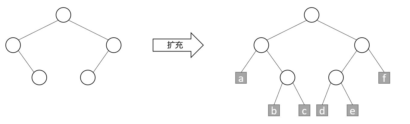
Consider a binary tree. It has a special kind of nodes called external nodes, which replace the empty subtree in the tree. The remaining nodes are called internal nodes. A binary tree with external nodes is called an extended binary tree. As shown in the figure, the gray box node represents the external node:

2. High priority left high tree

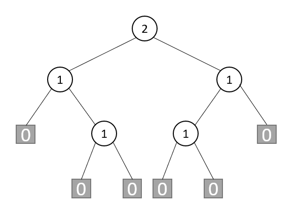
Let s(x) represent the shortest path from node x to the external node of its subtree. According to the definition of s(x), if x is an external node, the value of S is 0; If x is an internal node, the value of S is: m i n { s ( L ) , s ( R ) } + 1 min\{s(L),s(R)\}+1 min{s(L),s(R)}+1
Where, L and R are left and right children of x respectively. The s value of each node in the extended binary tree is shown in the figure:

(1) Definition

A binary tree is called high priority left height tree (HBLT), if and only if the s value of the left child of any internal node is greater than or equal to the s value of the right child.

The binary tree shown above is not HBLT. Considering the parent node of external node a, its left child's s s value is 0 and its right child's value is 1, although other internal nodes meet the definition of HBLT. If the left and right subtrees of the parent node of node a are exchanged, the tree becomes HBLT.

(2) Characteristics

If x is an internal node of HBLT, then:
① The number of nodes in the subtree with x as the root is at least 2 s ( x ) − 1 2^{s(x)}-1 2s(x)−1
② If the subtree with X as the root has m nodes, then s(x) is at most log ⁡ 2 ( m + 1 ) \log_2{(m+1)} log2​(m+1)
③ The length of the rightmost path from X to an external node is s(x).

(3) HBLT and size root tree

If a HBLT is also a large root tree, it is called the largest HBLT. If a HBLT is also a small root tree, it is called the minimum HBLT.
The maximum priority queue can be represented by the maximum HBLT, and the minimum priority queue can be represented by the minimum HBLT.

3. Weight first left high tree

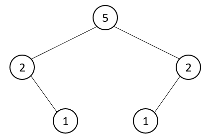
If we consider not the path length but the number of nodes, we can get another left height tree. The defined weight w(x) is the number of internal nodes of the subtree with node x as the root. If x is an external node, its weight is 0; If x is an internal node, its weight is the sum of the weights of its child nodes plus 1. The weight of each node in the extended binary tree is shown in the figure:

A binary tree is called weight first left height tree (WBLT), if and only if the w value of the left child of any internal node is greater than or equal to the w value of the right child. If a WBLT is also a large root tree, it is called the maximum WBLT. If a WBLT is also a small root tree, it is called the minimum WBLT.

Similar to HBLT, the rightmost path length of WBLT with m nodes is up to log ⁡ 2 ( m + 1 ) \log_2{(m+1)} log2​(m+1). Using WBLT or HBLT, the time complexity of finding, inserting and deleting portability priority queue is the same as that of heap. Like heap, WBLT and HBLT can complete initialization in linear time. Two priority queues represented by WBLT or HBLT can be combined into one in logarithmic time, but the priority queue represented by heap cannot do this.

Let's take HBLT as an example to introduce the implementation of related operations. WBLT is similar to it.

4. Insertion of maximum HBLT

The insert operation of the maximum HBLT can be realized by the merge operation of the maximum HBLT. Suppose the element x is inserted into the largest HBLT named H. If you build a maximum HBLT with only one element x and merge it with H, the merged maximum HBLT will contain all elements of H and element x. Therefore, to insert an element, you can first create a new HBLT containing only this element, and then merge the new HBLT with the original HBLT.

5. Deletion of maximum HBLT

The largest element is in the root. If the root is deleted, the subtrees with left and right children as the roots are the two largest HBLT. Merging the two largest HBLT is the result of deletion. Therefore, the deletion operation can be realized by merging the two subtrees after deleting the root element.

6. Merger of two largest HBLT

For HBLT with n elements, the length of the rightmost path is O ( l o g n ) O(log n) O(logn), an algorithm can only traverse its rightmost path to merge two HBLT. Since the time taken to implement the merge on each node is O ( 1 ) O(1) O(1), so the time complexity of the merging algorithm is the logarithm of the number of nodes after merging. Therefore, the algorithm starts from the roots of two HBLT trees and only moves along the right child.

The merge strategy is best implemented with recursion. Let A and B be the two largest HBLT to be merged. If one is empty, the other is the result of the merge. Assume that neither is empty. In order to merge, first compare the two root elements, and the larger one is the merged root. Suppose the root of A is large and the left subtree is L. Let C be the HBLT formed by merging the right subtree of A and B. The result of merging A and B is the maximum HBLT with A as the root and l and C as the subtree. If the s value of L is less than the s value of C, then C is the left subtree, otherwise L is the left subtree.

7. Initialization of HBLT

The initialization process is to insert n elements one by one into the maximum HBLT that was initially empty. The time required is O ( n l o g n ) O(nlog n) O(nlogn). In order to get the initialization algorithm with linear time, we first create n maximum HBLT with only one element, and the N trees form a FIFO queue, then delete HBLT from the queue in pairs, and then merge them and insert them at the end of the queue until there is only one HBLT in the queue.

2, Left high tree implementation

We implement the left high tree by inheriting the chain binary tree implemented earlier, because the left high tree does not need to store additional data.

1. Chained binary tree modification

Modifications to the linked binary tree include:
(1) Private member becomes protected member:

template<typename T>
class linkedBinaryTree : public binaryTree<T>
{
protected:
	binaryTreeNode<T>* root = nullptr;
	int treeSize = 0;
	std::function<void(T)> visitFunc;
	std::function<void(binaryTreeNode<T>*)> visitNodeFunc;
	...
}

(2) Extract the operation during destruct as clear function:

template<typename T>
inline void linkedBinaryTree<T>::clear()
{
	visitNodeFunc = [](binaryTreeNode<T>* node) {delete node; };
	postOrder(root);
	visitNodeFunc = std::function<void(binaryTreeNode<T>*)>();
}

2. Left high tree interface

The node type of the left high tree is STD:: pair < int, t >, the first member represents the s value of the node, and the second member represents the element itself.

#pragma once
#include <utility>
#include <stdexcept>
#include <queue>
#include <algorithm>
#include <functional>
#include <iostream>
#include "priorityQueue.h"
#include "../binaryTree/binaryTreeNode.h"
#include "../binaryTree/linkedBinaryTree.h"

template <typename T, typename Predicate = std::greater_equal<T>>
class hblt : public priorityQueue<T>, linkedBinaryTree<std::pair<int, T>>
{
public:
	using NodeType = binaryTreeNode<std::pair<int, T>>;

	virtual bool empty() const override;
	virtual int size() const override;
	virtual T& top() override;
	virtual void pop() override;
	virtual void push(const T& element) override;

	void meld(const hblt& other);
	void meld(hblt&& other);

	void initialize(T* origin, int arrayLength);
	void output();

private:
	void meld(NodeType* &left, NodeType* &right);

	void checkSize();

	int& nodePathLen(NodeType* node);
	T& nodeData(NodeType* node);
};

3. Left high tree merge private interface

All left height tree modification operations involve the function of left height tree merging. The previous algorithm has described most of this function. Finally, we need to update the node length of the merged tree root. The implementation is as follows:

template<typename T, typename Predicate>
inline void hblt<T, Predicate>::meld(NodeType* &left, NodeType* &right)
{
	using std::swap;

	if (left == nullptr)
	{
		left = right;
		return;
	}

	if (right == nullptr)
	{
		return;
	}

	Predicate pred;
	if (!pred(nodeData(left), nodeData(right)))
	{
		swap(left, right);
	}
	
	meld(left->rightChild, right);
	if (left->leftChild == nullptr || (left->rightChild != nullptr && nodePathLen(left->leftChild) < nodePathLen(left->rightChild)))
	{
		swap(left->leftChild, left->rightChild);
	}

	if (left->leftChild != nullptr)
	{
		nodePathLen(left) = nodePathLen(left->leftChild) + 1;
	}
	else
	{
		nodePathLen(left) = 1;
	}
}

template<typename T, typename Predicate>
inline int& hblt<T, Predicate>::nodePathLen(NodeType* node)
{
	return node->element.first;
}

template<typename T, typename Predicate>
inline T& hblt<T, Predicate>::nodeData(NodeType* node)
{
	return node->element.second;
}

4. Find maximum element

template<typename T, typename Predicate>
inline T& hblt<T, Predicate>::top()
{
	checkSize();
	return nodeData(this->root);
}

template<typename T, typename Predicate>
inline void hblt<T, Predicate>::checkSize()
{
	if (this->treeSize == 0)
	{
		throw std::overflow_error("no element in the tree");
	}
}

5. Element deletion

template<typename T, typename Predicate>
inline void hblt<T, Predicate>::pop()
{
	checkSize();

	auto rightChild = this->root->rightChild;
	auto leftChild = this->root->leftChild;
	delete this->root;

	this->root = this->root->leftChild;
	meld(this->root, rightChild);
	--this->treeSize;
}

6. Element insertion

template<typename T, typename Predicate>
inline void hblt<T, Predicate>::push(const T& element)
{
	auto tempRoot = new NodeType(std::make_pair(1, element));
	meld(this->root, tempRoot);
	++this->treeSize;
}

7. Left high tree merge

Here we provide two interfaces for movable trees and non movable trees respectively. The implementation in the tree moves a non const referenced tree, which is not a good choice. Using an R-value reference implies that we will directly use the data of the moved tree.

template<typename T, typename Predicate>
inline void hblt<T, Predicate>::meld(const hblt& other)
{
	auto tempTree = new hblt(other);
	meld(std::move(*tempTree));
	delete tempTree;
}

template<typename T, typename Predicate>
inline void hblt<T, Predicate>::meld(hblt&& other)
{
	meld(this->root, other.root);
	this->treeSize += other.treeSize;
	other.root = nullptr;
}

8. Initialization

template<typename T, typename Predicate>
inline void hblt<T, Predicate>::initialize(T* origin, int arrayLength)
{
	std::queue<NodeType*> meldNodes;
	std::for_each(origin, origin + arrayLength, [&meldNodes](T element) {meldNodes.push(new NodeType(std::make_pair(1, element))); });

	while (meldNodes.size() > 1)
	{
		auto left = meldNodes.front();
		meldNodes.pop();
		auto right = meldNodes.front();
		meldNodes.pop();

		meld(left, right);
		meldNodes.push(left);
	}

	if (!meldNodes.empty())
	{
		this->clear();
		this->treeSize = arrayLength;
		this->root = meldNodes.front();
		meldNodes.pop();
	}
}

9. Complexity analysis

The time complexity of the lookup function is O ( 1 ) O(1) O(1). The time complexity of inserting, deleting and merging is the same as that of the private method meld, which is essentially the merging of two binary trees. The private method meld moves only along the right subtree of left and right, so the complexity of this function is O ( s ( l e f t ) + s ( r i g h t ) ) = O ( l o g m + l o g n ) = O ( l o g n ) O(s(left)+s(right))=O(log m + log n)=O(log n) O(s(left)+s(right))=O(logm+logn)=O(logn).

When analyzing the complexity of the initialization function, for simplicity, assume that n is a power of 2. Merge first n 2 \frac{n}{2} 2n) for HBLT, each tree contains one element; Then merge n 4 \frac{n}{4} 4n# for HBLT, each tree contains 2 elements; Go on like this. If each tree contains 2 i 2^i 2i elements, then it takes time to merge the two largest HBLT trees O ( i + 1 ) O(i+1) O(i+1). Therefore, the total time taken by the initialize function is: O ( n 2 + 2 ∗ n 4 + ⋅ ⋅ ⋅ ) = O ( n ∑ i 2 i ) = O ( n ) O(\frac{n}{2}+2*\frac{n}{4}+···)=O(n\sum\frac{i}{2^i})=O(n) O(2n​+2∗4n​+⋅⋅⋅)=O(n∑2ii​)=O(n).

10. Mistakes in the book

This class book gives the test code, but does not give the output results. If we try to compile the code provided by the author, we will find that it is absolutely incompatible with our own compilation results. The reason is that the implementation of the merge function in the book is problematic. The problem is in line 68:

if (x->leftChild == NULL)
{
      x->leftChild = x->rightChild;
      x->rightChild = NULL;
      
      // Original implementation
      // x->element.first = 1;
      
      // After modification
      if (x->leftChild == NULL)
      {
          x->element.first = 1;
      }
      else
      {
          x->element.first = x->leftChild->element.first + 1;
      }
}

If the left subtree is empty, after assigning the right subtree to the left subtree, the judgment of the shortest path should depend on whether the new left subtree is empty, rather than dead 1