1. Preface
1.1 case introduction
In this case, pytoch is used to build a DenseNet network structure for image classification of fashion MNIST dataset. The analysis of this problem can be divided into data preparation, model establishment, training with training set and testing the effect of model with test set.
1.2 environment configuration
(1) operating system: Windows10
(2) compiler environment: PyCharm Community Edition 2021.2
(3) configuration environment: Pytorch1.7.1 + torchvision8.2 + CUDA11.3
1.3 module import
This case needs to import the following library files and related modules:
import numpy as np
import pandas as pd
from sklearn.metrics import accuracy_score, confusion_matrix, classification_report
import matplotlib.pyplot as plt
import seaborn as sns
import copy
import time
import torch
import torch.nn as nn
from torch.optim import Adam
import torch.utils.data as Data
from torchvision import transforms
from torchvision.datasets import FashionMNIST
2. Image data preparation
Before model establishment and training, first prepare the FashionMNIST data set, which can be directly read by using the FashionMNIST() function of datasets module in torchvision library. If there is no current data in the specified working folder, the data can be automatically downloaded from the network.
2.1 preparation of training verification set
The loading handler of the training validation set is packaged as the following train_data_process() function, which is used to import training data sets, and then use Data.DataLoader() function to define them as data loaders. Each batch will contain 64 samples. Through len() function, you can calculate the number of batches contained in the data loader and output the display train_ The loader contains 938 batches. It should be noted that the parameter shuffle = False indicates that the samples used by each batch in the loader are fixed, which is conducive to dividing the model into training set and verification set according to the number of iterations. At the same time, in order to observe the content of each image in the dataset, a batch image can be obtained and visualized to observe the data.
# Processing training set data
def train_data_process():
    # Load the FashionMNIST dataset
    train_data = FashionMNIST(root="./data/FashionMNIST",  # Data path
                              train=True,  # Use only training datasets
                              transform=transforms.Compose([transforms.Resize(size=96), transforms.ToTensor()]),  # Change the PIL.Image or numpy.array data type to torch.FloatTensor type
                                                                                                                   # The size is Channel * Height * Width, and the value range is reduced to [0.0, 1.0]
                              download=False,  # If the corresponding dataset is not downloaded, select True
                              )
    train_loader = Data.DataLoader(dataset=train_data,  # Incoming dataset
                                   batch_size=64,  # Number of samples per Batch
                                   shuffle=False,  # Do not reorder the dataset
                                   num_workers=0,  # Number of processes started to load data
                                   )
    print("The number of batch in train_loader:", len(train_loader))  # There are 938 batches in total, and each batch contains 64 training samples

    # Get the data of a Batch
    for step, (b_x, b_y) in enumerate(train_loader):
        if step > 0:
            break
    batch_x = b_x.squeeze().numpy()  # Remove the first dimension of the four-dimensional tensor and convert it into a Numpy array
    batch_y = b_y.numpy()  # Convert tensor to Numpy array
    class_label = train_data.classes  # Label of training set
    class_label[0] = "T-shirt"
    print("the size of batch in train data:", batch_x.shape)

    # Visualize an image of a Batch
    plt.figure(figsize=(12, 5))
    for ii in np.arange(len(batch_y)):
        plt.subplot(4, 16, ii+1)
        plt.imshow(batch_x[ii, :, :], cmap=plt.cm.gray)
        plt.title(class_label[batch_y[ii]], size=9)
        plt.axis("off")
        plt.subplots_adjust(wspace=0.05)
    plt.show()

    return train_loader, class_label
The obtained visual images are as follows:
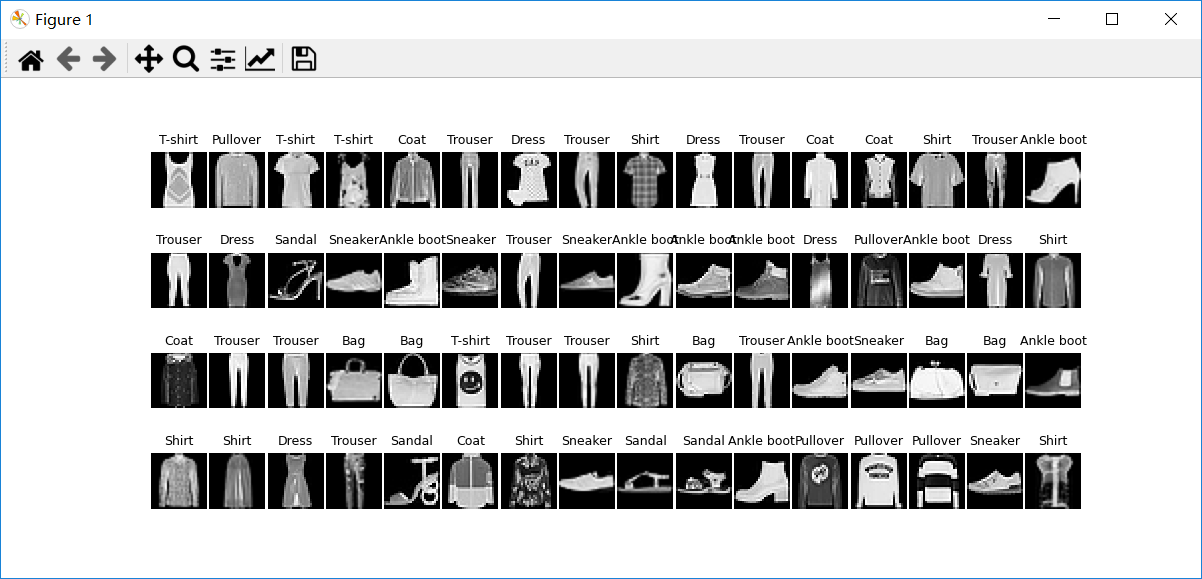
Note: since the input size of DenseNet model is 96, here we expand the size of fashion MNIST dataset to 96, and the size of each batch is 64, so the size of each mini batch is 64 × ninety-six × 96.
2.2 preparation of test set
The load handler for the test set is packaged as the following test_ data_ The process () function is used to import the test data set, expand its size to 96, and process all samples as a whole as a batch for testing..
# Processing test set data
def test_data_process():
    test_data = FashionMNIST(root="./data/FashionMNIST",  # Data path
                             train=False,  # Do not use training dataset
                             transform=transforms.Compose([transforms.Resize(size=96), transforms.ToTensor()]),  # Change the PIL.Image or numpy.array data type to torch.FloatTensor type
                                                                                                                  # The size is Channel * Height * Width, and the value range is reduced to [0.0, 1.0]
                             download=False,  # If the previous data has been downloaded, there is no need to download it again
                             )
    test_loader = Data.DataLoader(dataset=test_data,  # Incoming dataset
                                  batch_size=1,  # Number of samples per Batch
                                  shuffle=True,  # Do not reorder the dataset
                                  num_workers=0,  # Number of processes started to load data
                                   )

    # Get the data of a Batch
    for step, (b_x, b_y) in enumerate(test_loader):
        if step > 0:
            break
    batch_x = b_x.squeeze().numpy()  # Remove the first dimension of the four-dimensional tensor and convert it into a Numpy array
    batch_y = b_y.numpy()  # Convert tensor to Numpy array
    print("The size of batch in test data:", batch_x.shape)

    return test_loader
3. Construction of convolutional neural network
3.1 creation of dense blocks
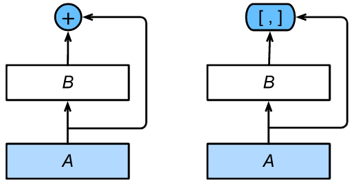
The main difference from ResNet is that the output of module B in DenseNet is not added to the output of module A like ResNet (as shown in the left part in the figure below), but connected in the channel dimension (as shown in the right part in the figure below), so that the output of module A can be directly transmitted to the layer behind module B. In this design, module A is directly connected with all layers behind module B, which is why it is called dense connection.
DenseNet uses the improved "batch normalization, activation and convolution" structure of ResNet. First, we_ This structure is implemented in the block () function.
# Define a convolution block
def conv_block(in_channels, out_channels):
    blk = nn.Sequential(nn.BatchNorm2d(in_channels),
                        nn.ReLU(),
                        nn.Conv2d(in_channels, out_channels, kernel_size=3, padding=1))

    return blk
Dense blocks consist of multiple convs_ Each block uses the same number of output channels. However, in forward calculation, we connect the input and output of each block in the channel dimension.
# Define a dense block
class DenseBlock(nn.Module):
    def __init__(self, num_convs, in_channels, out_channels):
        super(DenseBlock, self).__init__()
        net = []
        for i in range(num_convs):
            in_c = in_channels + i * out_channels
            net.append(conv_block(in_c, out_channels))
        self.net = nn.ModuleList(net)
        self.out_channels = in_channels + num_convs * out_channels  # Calculate the number of output channels

    def forward(self, X):
        for blk in self.net:
            Y = blk(X)
            X = torch.cat((X, Y), dim=1)  # Link input and output in channel dimension

        return X
3.2 creation of transition layer
Because each dense block will increase the number of channels, and excessive use will lead to too complex models, a transition layer is used to control the complexity of the model. It passes 1 × 1 convolution layer to reduce the number of channels, and use the average pool layer with step 2 to halve the height and width, so as to further reduce the complexity of the model.
# Define a transition layer
def transition_block(in_channels, out_channels):
    blk = nn.Sequential(nn.BatchNorm2d(in_channels),
                        nn.ReLU(),
                        nn.Conv2d(in_channels, out_channels, kernel_size=1),
                        nn.AvgPool2d(kernel_size=2, stride=2)
                        )

    return blk
3.3 establishment of densenet network
DenseNet first uses the same single volume layer and maximum pooling layer as ResNet. Next, DenseNet uses four dense blocks. Like ResNet, we can set how many convolution layers each dense block uses. This is set to 4, which is consistent with ResNet-18 in the previous article. The number of convolution layer channels (i.e. growth rate) in dense blocks is set to 32, so 128 channels will be added to each dense block. Use a transition layer between each dense block to halve the height and width and halve the number of channels. Finally, connect the global average pooling layer and the full connection layer to output.

# Define a global average pooling layer
class GlobalAvgPool2d(nn.Module):
    def __init__(self):
        super(GlobalAvgPool2d, self).__init__()

    def forward(self, x):
        return nn.functional.avg_pool2d(x, kernel_size=x.size()[2:])  # The pooled window shape is equal to the shape of the input image


# Define DenseNet network structure
def DenseNet(num_channels, growth_rate, num_convs_in_dense_blocks):
    net = nn.Sequential(nn.Conv2d(1, 64, kernel_size=7, stride=2, padding=3),
                        nn.BatchNorm2d(64),
                        nn.ReLU(),
                        nn.MaxPool2d(kernel_size=3, stride=2, padding=1)
                        )

    for i, num_convs in enumerate(num_convs_in_dense_blocks):
        DB = DenseBlock(num_convs, num_channels, growth_rate)
        net.add_module("DenseBlosk_%d" % i, DB)
        num_channels = DB.out_channels  # Number of output channels of the last dense block
        # A transition layer with half the number of channels is added between dense blocks
        if i != len(num_convs_in_dense_blocks) - 1:
            net.add_module("transition_block_%d" % i, transition_block(num_channels, num_channels // 2))
            num_channels = num_channels // 2

    net.add_module("BN", nn.BatchNorm2d(num_channels))
    net.add_module("relu", nn.ReLU())
    net.add_module("global_avg_pool", GlobalAvgPool2d())  # Output of GlobalAvgPool2d: (Batch, num_channels, 1, 1)
    net.add_module("fc", nn.Sequential(nn.Flatten(), nn.Linear(num_channels, 10)))

    return net
4. Convolutional neural network training and prediction
In order to train the network structure DenseNet, a train is defined_ Model() function, which is used to train DenseNet network with training data set. The training data set contains 60000 images and is divided into 938 batch es, of which 80% are used for model training and 20% for model verification_ The model () function includes two processes: model training and model verification.
# Define the training process of the network
def train_model(model, traindataloader, train_rate, criterion, device, optimizer, num_epochs=25):
    '''
    :param model: network model
    :param traindataloader: The training data set is divided into training set and verification set
    :param train_rate: Training set batch_size Percentage of
    :param criterion: loss function
    :param device: Operating equipment
    :param optimizer: optimization method
    :param num_epochs: Number of rounds of training
    '''

    batch_num = len(traindataloader)  # batch quantity
    train_batch_num = round(batch_num * train_rate)  # 80% of the batch is used for training, and the round() function is rounded
    best_model_wts = copy.deepcopy(model.state_dict())  # Copy parameters of the current model
    # Initialization parameters
    best_acc = 0.0  # Highest accuracy
    train_loss_all = []  # Training set loss function list
    train_acc_all = []  # Training set accuracy list
    val_loss_all = []  # Validation set loss function list
    val_acc_all = []  # Validation set accuracy list
    since = time.time()  # current time
    # Iterative training model
    for epoch in range(num_epochs):
        print('Epoch {}/{}'.format(epoch, num_epochs - 1))
        print('-' * 10)

        # Initialization parameters
        train_loss = 0.0  # Training set loss function
        train_corrects = 0  # Training set accuracy
        train_num = 0  # Number of training set samples
        val_loss = 0.0  # Verification set loss function
        val_corrects = 0  # Verification set accuracy
        val_num = 0  # Number of validation set samples
        # Train and calculate each mini batch
        for step, (b_x, b_y) in enumerate(traindataloader):
            b_x = b_x.to(device)
            b_y = b_y.to(device)
            if step < train_batch_num:  # 80% of the data set was used for training
                model.train()  # Set the model to training mode and enable Batch Normalization and Dropout
                output = model(b_x)  # In the forward propagation process, the input is a batch and the output is the corresponding prediction in a batch
                pre_lab = torch.argmax(output, 1)  # Find the row mark corresponding to the maximum value in each row
                loss = criterion(output, b_y)  # Calculate the loss function of each batch
                optimizer.zero_grad()  # Initialize gradient to 0
                loss.backward()  # Back propagation calculation
                optimizer.step()  # The network parameters are updated according to the gradient information of network back propagation to reduce the calculated value of loss function
                train_loss += loss.item() * b_x.size(0)  # Accumulate the loss function
                train_corrects += torch.sum(pre_lab == b_y.data)  # If the prediction is correct, the accuracy train_ Correct plus 1
                train_num += b_x.size(0)  # Number of samples currently used for training
            else:  # Use 20% of the dataset for validation
                model.eval()  # Set the model to evaluation mode and do not enable Batch Normalization and Dropout
                output = model(b_x)  # In the forward propagation process, the input is a batch and the output is the corresponding prediction in a batch
                pre_lab = torch.argmax(output, 1)  # Find the row mark corresponding to the maximum value in each row
                loss = criterion(output, b_y)  # Calculate the average loss function of 64 samples in each batch
                val_loss += loss.item() * b_x.size(0)  # Accumulate the loss function of each batch in the validation set
                val_corrects += torch.sum(pre_lab == b_y.data)  # If the prediction is correct, the accuracy val_ Correct plus 1
                val_num += b_x.size(0)  # Number of samples currently used for validation

        # Calculate and save the cost function and accuracy of each iteration
        train_loss_all.append(train_loss / train_num)  # Calculate and save the cost function of the training set
        train_acc_all.append(train_corrects.double().item() / train_num)  # Calculate and save the accuracy of the training set
        val_loss_all.append(val_loss / val_num)  # Calculate and save the cost function of the validation set
        val_acc_all.append(val_corrects.double().item() / val_num)  # Calculate and save the accuracy of the validation set
        print('{} Train Loss: {:.4f} Train Acc: {:.4f}'.format(epoch, train_loss_all[-1], train_acc_all[-1]))
        print('{} Val Loss: {:.4f} Val Acc: {:.4f}'.format(epoch, val_loss_all[-1], val_acc_all[-1]))

        # Find the highest accuracy
        if val_acc_all[-1] > best_acc:
            best_acc = val_acc_all[-1]  # Save current maximum accuracy
            best_model_wts = copy.deepcopy(model.state_dict())  # Save the model parameters at the current highest accuracy
        time_use = time.time() - since  # Computing takes time
        print("Train and val complete in {:.0f}m {:.0f}s".format(time_use // 60, time_use % 60))

    # Select the optimal parameters
    model.load_state_dict(best_model_wts)  # Load the model parameters at the highest accuracy
    train_process = pd.DataFrame(data={"epoch": range(num_epochs),
                                       "train_loss_all": train_loss_all,
                                       "val_loss_all": val_loss_all,
                                       "train_acc_all": train_acc_all,
                                       "val_acc_all": val_acc_all}
                                 )  # Save the loss function and accuracy of each generation in DataFrame format

    # The loss function and accuracy of the training set and verification set after each iteration are displayed
    plt.figure(figsize=(12, 4))
    plt.subplot(1, 2, 1)
    plt.plot(train_process['epoch'], train_process.train_loss_all, "ro-", label="Train loss")
    plt.plot(train_process['epoch'], train_process.val_loss_all, "bs-", label="Val loss")
    plt.legend()
    plt.xlabel("epoch")
    plt.ylabel("Loss")
    plt.subplot(1, 2, 2)
    plt.plot(train_process['epoch'], train_process.train_acc_all, "ro-", label="Train acc")
    plt.plot(train_process['epoch'], train_process.val_acc_all, "bs-", label="Val acc")
    plt.xlabel("epoch")
    plt.ylabel("acc")
    plt.legend()
    plt.show()

    return model, train_process
Next, define a test_model() function, which is used to test on the optimal model using the test set, so as to verify the performance of the model.
# test model
def test_model(model, testdataloader, device):
    '''
    :param model: network model
    :param testdataloader: Test data set
    :param device: Operating equipment
    '''

	# Initialization parameters
    test_corrects = 0.0
    test_num = 0
    test_acc = 0.0
    # Only forward propagation calculation is performed without gradient calculation, so as to save memory and speed up operation
    with torch.no_grad():
        for test_data_x, test_data_y in testdataloader:
            test_data_x = test_data_x.to(device)
            test_data_y = test_data_y.to(device)
            model.eval()  # Set the model to evaluation mode and do not enable Batch Normalization and Dropout
            output = model(test_data_x)  # In the forward propagation process, the input is the test data set and the output is the prediction of each sample
            pre_lab = torch.argmax(output, 1)  # Find the row mark corresponding to the maximum value in each row
            test_corrects += torch.sum(pre_lab == test_data_y.data)  # If the prediction is correct, the accuracy val_ Correct plus 1
            test_num += test_data_x.size(0)  # Number of samples currently used for training

    test_acc = test_corrects.double().item() / test_num  # Calculate the classification accuracy on the test set
    print("test accuracy:", test_acc)
Finally, the model is trained and tested. The optimization algorithm uses Adam optimizer, the learning rate is set to 0.001, and the loss function is the cross entropy function. Then call train_. The model() function trains the training set train_ 80% of the loader is used for training and 20% for verification, with a total of 25 rounds of training.
# Model training and testing
def train_model_process(myconvnet):
    optimizer = torch.optim.Adam(myconvnet.parameters(), lr=0.001)  # Using Adam optimizer, the learning rate is 0.001
    criterion = nn.CrossEntropyLoss()  # The loss function is the cross entropy function
    device = 'cuda' if torch.cuda.is_available() else 'cpu'  # GPU acceleration
    train_loader, class_label = train_data_process()  # Load training set
    test_loader = test_data_process()  # Load test set

    myconvnet = myconvnet.to(device)
    myconvnet, train_process = train_model(myconvnet, train_loader, 0.8, criterion, device, optimizer, num_epochs=25)  # Start training model
    test_model(myconvnet, test_loader, device)  # Evaluation using test sets
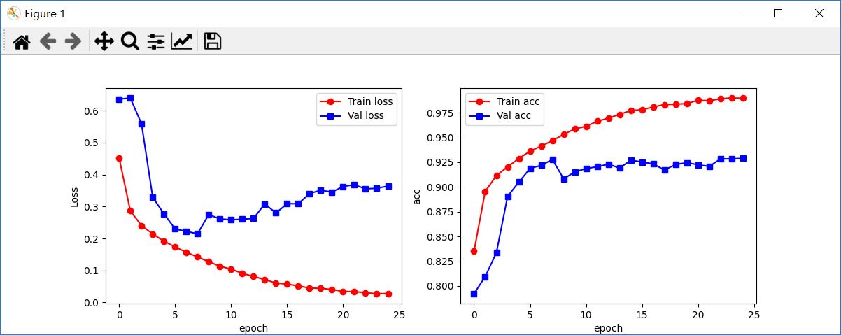
In the process of model training, the change curves of loss function and classification accuracy are as follows. It can be seen that the loss function decreases rapidly in the training set, decreases rapidly in the verification set, and then fluctuates and increases slightly. The classification accuracy has been increasing in the training set, and began to fluctuate slightly after gradually increasing in the verification set.
In order to obtain the generalization ability of the calculation model, the test set is given to the trained model for prediction, so as to obtain the prediction accuracy on the test set (as shown in the figure below).

Note: for complex neural networks and large-scale data, using CPU to calculate may not be efficient enough. Therefore, it is necessary to move the model to GPU and use GPU to accelerate calculation.
5. Operation procedure
The following is the content of the main function, configure parameters and return a DenseNet network structure, and then train and test the convolutional neural network.
if __name__ == '__main__':
    num_channels, growth_rate = 64, 32  # num_channels is the current number of channels
    num_convs_in_dense_blocks = [4, 4, 4, 4]
    model = DenseNet(num_channels, growth_rate, num_convs_in_dense_blocks)
    train_model_process(model)
Note: in the previous program, it is configured to use multiple processes to load training set data at the same time. The use of multiple processes must be carried out in the main() function, otherwise an error will be reported during execution.