1, Introduction to particle swarm optimization

Particle swarm optimization algorithm was proposed by Dr. Eberhart and Dr. Kennedy in 1995. It comes from the study of bird predation behavior. Its basic core is to make use of the information sharing of individuals in the group, so as to make the movement of the whole group produce an evolutionary process from disorder to order in the problem-solving space, so as to obtain the optimal solution of the problem. Imagine this scenario: a flock of birds are foraging, and there is a corn field in the distance. All the birds don't know where the corn field is, but they know how far their current position is from the corn field. Then the best strategy to find the corn field, and the simplest and most effective strategy, is to search the surrounding area of the nearest bird group to the corn field.

In PSO, the solution of each optimization problem is a bird in the search space, which is called "particle", and the optimal solution of the problem corresponds to the "corn field" found in the bird swarm. All particles have a position vector (the position of the particle in the solution space) and a velocity vector (which determines the direction and speed of the next flight), and the fitness value of the current position can be calculated according to the objective function, which can be understood as the distance from the "corn field". In each iteration, the examples in the population can learn not only according to their own experience (historical position), but also according to the "experience" of the optimal particles in the population, so as to determine how to adjust and change the flight direction and speed in the next iteration. In this way, the whole population will gradually tend to the optimal solution.

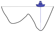
The above explanation may be more abstract. Let's illustrate it with a simple example

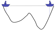
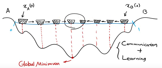
There are two people in a lake. They can communicate with each other and detect the lowest point of their position. The initial position is shown in the figure above. Because the right side is deep, the people on the left will move the boat to the right.

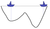
Now the left side is deep, so the person on the right will move the boat to the left

Keep repeating the process and the last two boats will meet

A local optimal solution is obtained

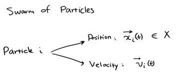
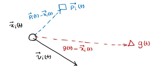
Represent each individual as a particle. The position of each individual at a certain time is expressed as x(t), and the direction is expressed as v(t)

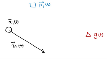
p (T) is the optimal solution of individual x at time t, g(t) is the optimal solution of all individuals at time t, v(t) is the direction of individual at time t, and x(t) is the position of individual at time t

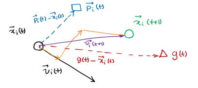
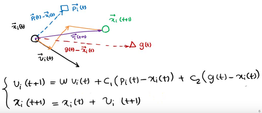
The next position is shown in the figure above, which is determined by X, P and G

The particles in the population can find the optimal solution of the problem by constantly learning from the historical information of themselves and the population.

However, in the follow-up research, the table shows that there is a problem in the above original formula: the update of V in the formula is too random, which makes the global optimization ability of the whole PSO algorithm strong, but the local search ability is poor. In fact, we need that PSO has strong global optimization ability in the early stage of algorithm iteration, and the whole population should have stronger local search ability in the later stage of algorithm iteration. Therefore, according to the above disadvantages, shi and Eberhart modified the formula by introducing inertia weight, so as to put forward the inertia weight model of PSO:

The components of each vector are represented as follows

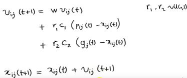
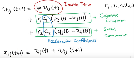
Where W is called the inertia weight of PSO, and its value is between [0,1]. Generally, adaptive value method is adopted, that is, w=0.9 at the beginning, which makes PSO have strong global optimization ability. With the deepening of iteration, the parameter W decreases, so that PSO has strong local optimization ability. When the iteration is over, w=0.1. The parameters c1 and c2 are called learning factors and are generally set to 14961; r1 and r2 are random probability values between [0,1].

The algorithm framework of the whole particle swarm optimization algorithm is as follows:

Step 1 population initialization can be carried out randomly or design a specific initialization method according to the optimized problem, and then calculate the individual fitness value, so as to select the individual local optimal position vector and the global optimal position vector of the population.

Step 2 iteration setting: set the number of iterations and set the current number of iterations to 1

step3 speed update: update the speed vector of each individual

step4 position update: update the position vector of each individual

Step 5 local position and global position vector update: update the local optimal solution of each individual and the global optimal solution of the population

Step 6 termination condition judgment: the maximum number of iterations is reached when judging the number of iterations. If it is satisfied, the global optimal solution is output. Otherwise, continue the iteration and jump to step 3.

For the application of particle swarm optimization algorithm, it is mainly the design of velocity and position vector iterative operators. Whether the iterative operator is effective or not will determine the performance of the whole PSO algorithm, so how to design the iterative operator of PSO is the research focus and difficulty in the application of PSO algorithm.

2, VRP model

(1) Introduction to vehicle path planning

After 60 years of research and development, the research objectives and constraints of vehicle routing problem have changed. It has changed from the initial simple vehicle scheduling problem to a complex system problem. The initial vehicle path planning problem can be described as: there is a starting point and several customer points. Given the geographical location and needs of each point, how to plan the optimal path under the conditions of meeting various constraints, so that it can serve each customer point, and finally return to the starting point. By imposing different constraints and changing the optimization objectives, different kinds of vehicle routing problems can be derived. At the same time, the vehicle routing problem belongs to a typical NP hard problem, and its exact algorithm can solve a small scale, so the heuristic algorithm has become a research hotspot.

(2) Introduction to VRPTW

VRPTW(Vehicle routing problem with time windows) is a vehicle routing problem with time window. It adds time window constraints to each demand point, that is, for each demand point, set the earliest and latest time of service start, and require the vehicle to start serving customers within the time window.

There are two kinds of time window restrictions at the demand point. One is the hard time window, which requires the vehicle to start serving customers within the time window, wait early and reject it if it is late. The other is the soft time window, which does not necessarily start serving customers within the time window, but must be punished if it starts serving outside the time window, Penalty instead of waiting and rejection is the biggest difference between soft time window and hard time window.

The mathematical model of VRPTW is as follows:

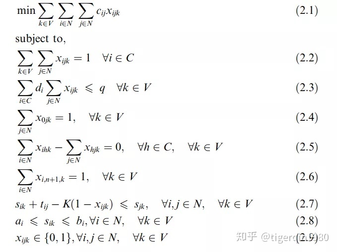
(2.2) ensure that each customer is only visited once

(2.3) ensure that the loaded goods do not exceed the capacity

(2.4) (2.5) (2.6) ensure that each vehicle starts from the depot and finally returns to the depot

(2.7) (2.8) ensure that the service starts within the time window

3, Code

clc %Clear command line window
clear %Deletes all variables from the current workspace and frees them from system memory
close all %Delete all windows whose handles are not hidden
tic % Save current time
%% GA-PSO Algorithm solving CDVRP
%Input:
%City           Longitude and latitude of demand point
%Distance       Distance matrix
%Demand         Demand at each point
%Travelcon      Travel constraint
%Capacity       Vehicle capacity constraint
%NIND           Population number
%MAXGEN         Inherited to the third MAXGEN Time substitution program stop

%Output:
%Gbest          Shortest path
%GbestDistance	Shortest path length

%% Load data
load('../test_data/City.mat')	      %The longitude and latitude of the demand point is used to draw the actual path XY coordinate
load('../test_data/Distance.mat')	  %Distance matrix
load('../test_data/Demand.mat')       %requirement
load('../test_data/Travelcon.mat')	  %Travel constraint
load('../test_data/Capacity.mat')     %Vehicle capacity constraint

%% Initialize problem parameters
CityNum=size(City,1)-1; %Number of demand points

%% Initialization algorithm parameters
NIND=60; %Number of particles
MAXGEN=100; %Maximum number of iterations

%% 0 matrix initialized for pre allocated memory
Population = zeros(NIND,CityNum*2+1); %Pre allocated memory for storing population data
PopDistance = zeros(NIND,1); %Pre allocated matrix memory
GbestDisByGen = zeros(MAXGEN,1); %Pre allocated matrix memory

for i = 1:NIND
    %% Initialize each particle
    Population(i,:)=InitPop(CityNum,Distance,Demand,Travelcon,Capacity); %Random generation TSP route
    
    %% Calculate path length
    PopDistance(i) = CalcDis(Population(i,:),Distance,Demand,Travelcon,Capacity); % Calculate path length
end

%% storage Pbest data
Pbest = Population; % initialization Pbest For the current particle collection
PbestDistance = PopDistance; % initialization Pbest The objective function value of is the objective function value of the current particle collection

%% storage Gbest data
[mindis,index] = min(PbestDistance); %get Pbest in
Gbest = Pbest(index,:); % initial Gbest particle
GbestDistance = mindis; % initial Gbest Objective function value of particle

%% Start iteration
gen=1;

while gen <= MAXGEN
    %% Update per particle
    for i=1:NIND
        %% Particles and Pbest overlapping
        Population(i,2:end-1)=Crossover(Population(i,2:end-1),Pbest(i,2:end-1)); %overlapping
        
        % If the length of the new path becomes shorter, record to Pbest
        PopDistance(i) = CalcDis(Population(i,:),Distance,Demand,Travelcon,Capacity); %Calculate distance
        if PopDistance(i) < PbestDistance(i) %If the length of the new path becomes shorter
            Pbest(i,:)=Population(i,:); %to update Pbest
            PbestDistance(i)=PopDistance(i); %to update Pbest distance
        end

    %% Update iterations
    gen=gen+1;
end

%Delete redundant 1 in path
for i=1:length(Gbest)-1
    if Gbest(i)==Gbest(i+1)
        Gbest(i)=0;  %When the adjacent bits are all 1, the previous one is set to zero
    end
end
Gbest(Gbest==0)=[];  %Delete redundant zero elements

Gbest=Gbest-1;  % Subtract 1 from each code, which is consistent with the code in the text

%% The calculation result data is output to the command line
disp('-------------------------------------------------------------')
toc %Display run time
fprintf('Total Distance = %s km \n',num2str(GbestDistance))
TextOutput(Gbest,Distance,Demand,Capacity)  %Show optimal path
disp('-------------------------------------------------------------')

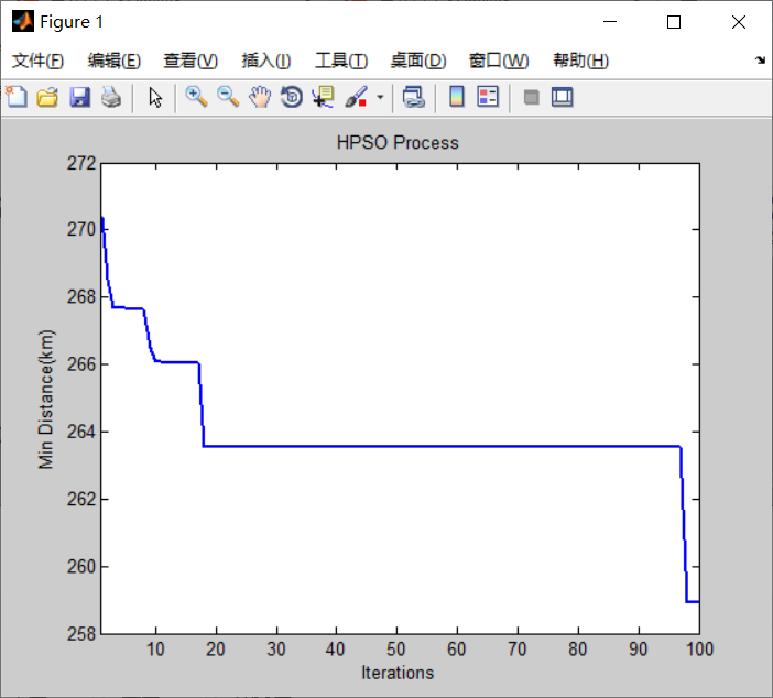
%% Iterative graph
figure
plot(GbestDisByGen,'LineWidth',2) %Show the historical change of objective function value
xlim([1 gen-1]) %set up x Axis range
set(gca, 'LineWidth',1)
xlabel('Iterations')
ylabel('Min Distance(km)')
title('HPSO Process')

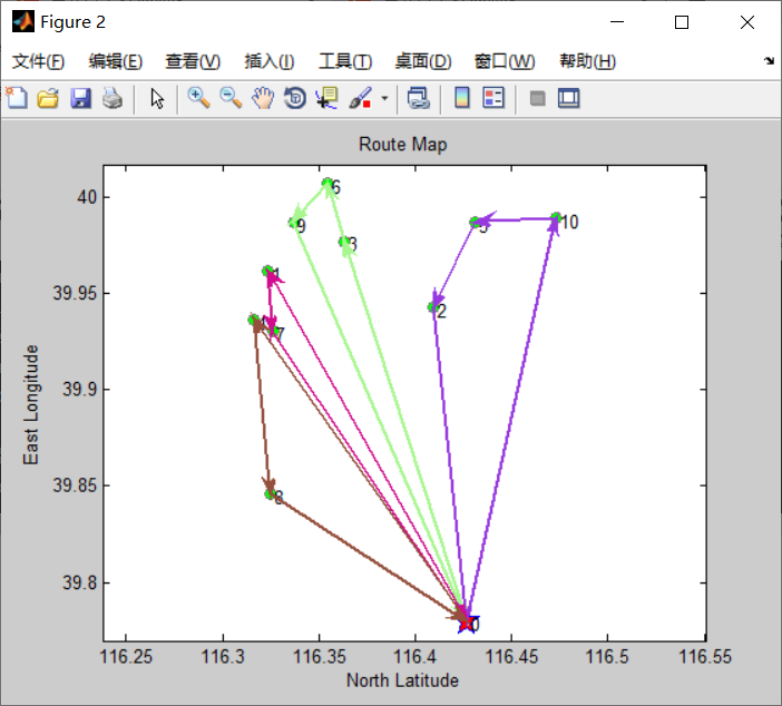
%% Draw actual route
DrawPath(Gbest,City)

4, Results