1. Introduction to Particle Swarm Optimization

Particle swarm optimization (PSO) was proposed by Dr. Eberhart and Dr. Kennedy in 1995. It originated from the study of bird predation behavior.Its basic core is to make use of the sharing of information by individuals in the group so that the movement of the whole group can evolve from disorder to order in the problem solving space, and obtain the optimal solution of the problem.Imagine a scene where a group of birds are feeding and there is a corn field in the distance. All the birds don't know where the corn field is, but they know how far away they are from it.The easiest and most effective strategy for finding a maize field is to search the area around the nearest flock of birds.

In PSO, the solution of each optimization problem is a bird in the search space, called a "particle", and the optimal solution of the problem corresponds to the "corn field" found in the bird population.All particles have a position vector (the location of the particle in the solution space) and a velocity vector (which determines the direction and speed of the next flight), and the fitness value of the current location can be calculated from the objective function, which can be interpreted as the distance from the "corn field".In each iteration, in addition to learning from their own experience (historical location), examples in the population can also be learned from the "experience" of the best particles in the population to determine how to adjust and change the direction and speed of flight in the next iteration.So iterate over time, and the final example of the entire population will gradually reach the optimal solution.

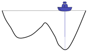
The above explanation may be abstract, but here is a simple example

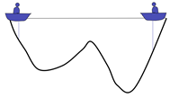
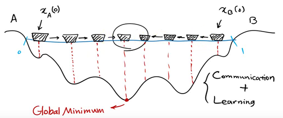
Two people in a lake can communicate with each other and detect the lowest point of their location.The initial position is shown in the figure above. Because the right side is deeper, the person on the left will move the boat a little to the right.

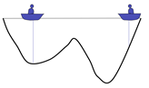
Now the left side is deeper, so the person on the right will move the boat to the left

Repeat the process until the last two boats meet

Get a local optimal solution

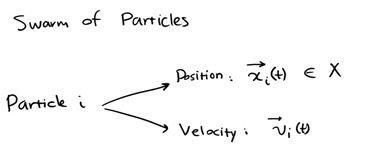
Represents each individual as a particle.Each individual's position at a time is expressed as x(t), and its direction is expressed as v(t)

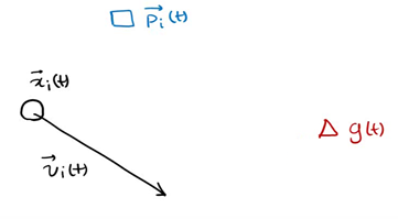
p(t) is the best solution for an individual at time x, g(t) is the best solution for all individuals at time t, v(t) is the direction of the individual at time t, and x(t) is the position of the individual at time t.

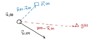
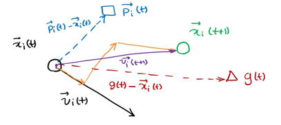
The next position is determined by x,p,g as shown in the figure above

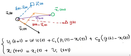
Particles in a population learn from themselves and the history of the population to find the best solution to the problem.

However, in subsequent studies, the table shows that there is a problem with the original formula mentioned above: the update of V in the formula is too random, which makes the PSO algorithm strong in global optimization, but poor in local search.In fact, we need PSO to have strong global optimization capability at the beginning of algorithm iteration, and the whole population should have stronger local search capability at the later stage of algorithm iteration.Therefore, according to the above drawbacks, shi and Eberhart modified the formula by introducing the inertia weight, thus putting forward the inertia weight model of PSO:

The scales for each vector are expressed as follows

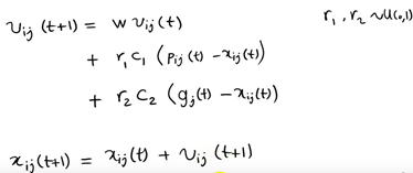
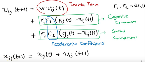
W is called the inertial weight of PSO, and its value is between [0,1]. In general, the adaptive value method is used in applications, that is, starting with w=0.9, which makes PSO have a strong global optimization ability. As the iteration goes deeper, the parameter w decreases, so that PSO has a strong local optimization ability. When the iteration ends, w=0.1.The parameters c1 and c2 are called learning factors and are generally set to 1,4961.R 1 and r2 are random probability values between [0,1].

The algorithm framework for the entire particle swarm optimization algorithm is as follows:

step1 population initialization can be done randomly or a specific initialization method can be designed according to the optimized problem, and then the fitness value of the individual is calculated to select the local optimal location vector of the individual and the global optimal location vector of the population.

Step 2 Iteration Settings: Set the number of iterations and make the current number of iterations 1

Step 3 Speed Update: Update each individual's speed vector

Step 4 Location Update: Update each individual's location vector

step5 local and global location vector updates: updating the local optimal solution for each individual and the global optimal solution for the population

step6 termination condition judgment: the maximum number of iterations is reached when the number of iterations is judged, if satisfied, the output global optimal solution, otherwise continue iteration, jump to step 3.

For the use of particle swarm optimization algorithm, the design of velocity and position vector iteration operator is the main focus.Whether the iteration operator is effective or not will determine the performance of the entire PSO algorithm, so how to design the iteration operator of the PSO is the research focus and difficulty of the application of the PSO algorithm.

2. TSP Model

3. Code

clc %Empty Command Line Window
clear %Remove all variables from the current workspace and free them from system memory
close all %Delete all windows whose handles are not hidden
tic % Save the current time
%% GA-PSO Algorithmic Solution TSP
%Input:
%City           Latitude and longitude of demand points
%Distance       Distance Matrix
%NIND           Number of Populations
%MAXGEN         Inherited to MAXGEN Timer Stop

%Output:
%Gbest          Shortest path
%GbestDistance	Shortest path length
%% Loading data
load('../test_data/City.mat')	      %Latitude and longitude of demand points, used to draw actual paths XY coordinate
load('../test_data/Distance.mat')	  %Distance Matrix

%% Initialization problem parameters
CityNum=size(City,1)-1; %Number of Demand Points

%% Initialization algorithm parameters
NIND=60; %Number of particles
MAXGEN=100; %Maximum number of iterations

%% Matrix 0 initialized for pre-allocating memory
Population = zeros(NIND,CityNum+2); %Preallocated memory for storing population data
PopDistance = zeros(NIND,1); %Preallocate Matrix Memory
GbestDisByGen = zeros(MAXGEN,1); %Preallocated matrix memory for drawing iteration diagrams

for i = 1:NIND
    %% Initialize particles
    Population(i,2:end-1)=InitPop(CityNum); %Random Generation TSP Route
    
    %% Calculate Path Length
    PopDistance(i) = CalcDis(Population(i,:),Distance); % Calculate Path Length
end

%% storage Pbest data
Pbest = Population; % Initialization Pbest For the current particle collection
PbestDistance = PopDistance; % Initialization Pbest The target function value is the target function value of the current particle set

%% storage Gbest data
[mindis,index] = min(PbestDistance); %Get Pbest Minimum value in
Gbest = Pbest(index,:); % initial Gbest particle
GbestDistance = mindis; % initial Gbest Target function value of particles

%% Start Iteration
gen=1;

while gen <= MAXGEN
    %% Update per Particle
    for i=1:NIND
        %% Particle and Pbest overlapping
        Population(i,2:end-1)=Crossover(Population(i,2:end-1),Pbest(i,2:end-1)); %overlapping
        
        % Shorter new path length is recorded to Pbest
        PopDistance(i) = CalcDis(Population(i,:),Distance); %Calculate Distance
        if PopDistance(i) < PbestDistance(i) %If the new path length is shorter
            Pbest(i,:)=Population(i,:); %To update Pbest
            PbestDistance(i)=PopDistance(i); %To update Pbest distance
        end
        

    end
    
    %% Show this generation of information
    fprintf('Iteration = %d, Min Distance = %.2f km  \n',gen,GbestDistance)
    
	%% Store the shortest distance of this generation
    GbestDisByGen(gen)=GbestDistance;
    
    %% Number of update iterations
    gen=gen+1;
end

%% Results of calculation are output to the command line
disp('-------------------------------------------------------------')
toc %Show run time
TextOutput(Gbest,GbestDistance)  %Show Optimal Path

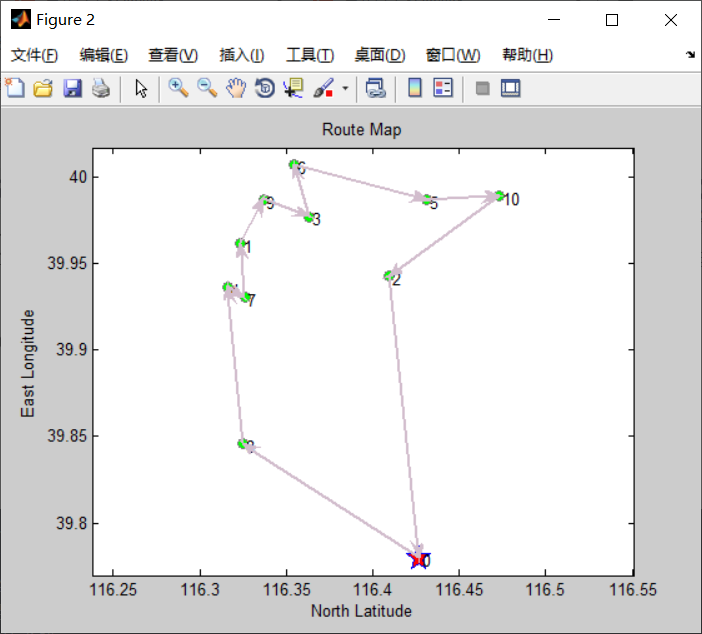
%% Iteration Diagram
figure
plot(GbestDisByGen,'LineWidth',2) %Show historical changes in objective function values
xlim([1 gen-1]) %Set up x Coordinate axis range
set(gca, 'LineWidth',1)
xlabel('Iterations')
ylabel('Min Distance(km)')
title('HPSO Process')

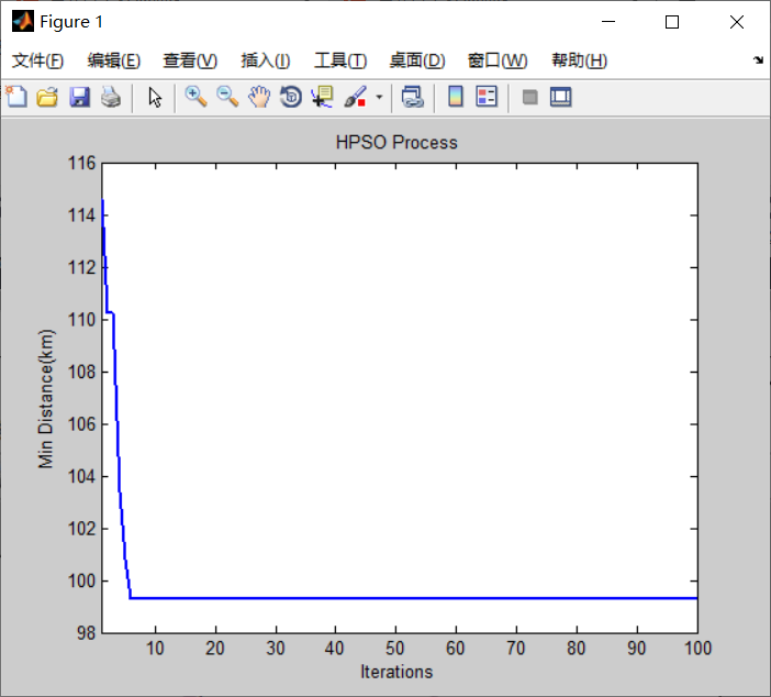
%% Draw the actual route
DrawPath(Gbest,City)