Why is resnet input certain?
Because resnet finally has a full connection layer. Because of this full connection layer, the size of the input image must be fixed.
What are the limitations of a fixed input size?
The original resnet will scale the image to 224 × 224 on the imagenet dataset, but there are some limitations in doing so:
(1) When the target object occupies a very small position in the image, scaling the image will further reduce the size of the object in the image, and the image may not be classified correctly
(2) When the image is not square or the object is not in the center of the image, scaling will cause the image to deform
(3) If you use the sliding window method to find the target object, this operation is expensive
How to modify resnet to fit different input sizes?
(1) Customize a network class of your own, but you need to inherit models.ResNet
(2) Replacing adaptive average pooling with normal average pooling
(3) Replace full connection layer with roll up layer
Related code:
import torch
import torch.nn as nn
from torchvision import models
import torchvision.transforms as transforms
from torch.hub import load_state_dict_from_url

from PIL import Image
import cv2
import numpy as np
from matplotlib import pyplot as plt

class FullyConvolutionalResnet18(models.ResNet):
    def __init__(self, num_classes=1000, pretrained=False, **kwargs):

        # Start with standard resnet18 defined here
        super().__init__(block = models.resnet.BasicBlock, layers = [2, 2, 2, 2], num_classes = num_classes, **kwargs)
        if pretrained:
            state_dict = load_state_dict_from_url( models.resnet.model_urls["resnet18"], progress=True)
            self.load_state_dict(state_dict)

        # Replace AdaptiveAvgPool2d with standard AvgPool2d
        self.avgpool = nn.AvgPool2d((7, 7))

        # Convert the original fc layer to a convolutional layer.
        self.last_conv = torch.nn.Conv2d( in_channels = self.fc.in_features, out_channels = num_classes, kernel_size = 1)
        self.last_conv.weight.data.copy_( self.fc.weight.data.view ( *self.fc.weight.data.shape, 1, 1))
        self.last_conv.bias.data.copy_ (self.fc.bias.data)

    # Reimplementing forward pass.
    def _forward_impl(self, x):
        # Standard forward for resnet18
        x = self.conv1(x)
        x = self.bn1(x)
        x = self.relu(x)
        x = self.maxpool(x)

        x = self.layer1(x)
        x = self.layer2(x)
        x = self.layer3(x)
        x = self.layer4(x)
        x = self.avgpool(x)

        # Notice, there is no forward pass
        # through the original fully connected layer.
        # Instead, we forward pass through the last conv layer
        x = self.last_conv(x)
        return x
It should be noted that we have copied the parameters of the full connection layer into our own defined convolution layer.
Take a look at the network structure, focusing on the last part of the network:
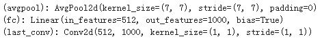
We will self.avgpool Instead of AvgPool2d, the full connection layer is still in the network, but it is not used in forward propagation.
Now we have this image:
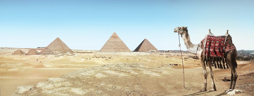
The image size is: (387, 1024, 3). And the target camel is in the lower right corner of the image.
Let's use this picture to see how to use it.
with open('imagenet_classes.txt') as f:
    labels = [line.strip() for line in f.readlines()]

# Read image
original_image = cv2.imread('camel.jpg')# Convert original image to RGB format
image = cv2.cvtColor(original_image, cv2.COLOR_BGR2RGB)

# Transform input image
# 1. Convert to Tensor
# 2. Subtract mean
# 3. Divide by standard deviation

transform = transforms.Compose([
              transforms.ToTensor(), #Convert image to tensor.
              transforms.Normalize(
              mean=[0.485, 0.456, 0.406],   # Subtract mean
              std=[0.229, 0.224, 0.225]     # Divide by standard deviation
              )])

image = transform(image)
image = image.unsqueeze(0)
# Load modified resnet18 model with pretrained ImageNet weights
model = fcresnet18.FullyConvolutionalResnet18(pretrained=True).eval()
print(model)
with torch.no_grad():
    # Perform inference.
    # Instead of a 1x1000 vector, we will get a
    # 1x1000xnxm output ( i.e. a probabibility map
    # of size n x m for each 1000 class,
    # where n and m depend on the size of the image.)
    preds = model(image)
    preds = torch.softmax(preds, dim=1)

    print('Response map shape : ', preds.shape)

    # Find the class with the maximum score in the n x m output map
    pred, class_idx = torch.max(preds, dim=1)
    print(class_idx)

    row_max, row_idx = torch.max(pred, dim=1)
    col_max, col_idx = torch.max(row_max, dim=1)
    predicted_class = class_idx[0, row_idx[0, col_idx], col_idx]

    # Print top predicted class
    print('Predicted Class : ', labels[predicted_class], predicted_class)
Description: imagenet_classes.txt Is the label information in. During data enhancement, the image was not resized. The format of the image read by opencv is BGR, and we need to convert it to the format of pytorch: RGB. At the same time, you need to use unsqueeze(0) to add a dimension, which becomes [batchsize,channel,height,width]. Take a look at avgpool and last_ Dimensions of conv's output:
We use the torchsummary library to view the output of each layer:
device = torch.device("cuda" if torch.cuda.is_available() else "cpu")
model.to(device)
from torchsummary import summary
summary(model, (3, 387, 1024))
result:
----------------------------------------------------------------
        Layer (type)               Output Shape         Param #
================================================================
            Conv2d-1         [-1, 64, 194, 512]           9,408
       BatchNorm2d-2         [-1, 64, 194, 512]             128
              ReLU-3         [-1, 64, 194, 512]               0
         MaxPool2d-4          [-1, 64, 97, 256]               0
            Conv2d-5          [-1, 64, 97, 256]          36,864
       BatchNorm2d-6          [-1, 64, 97, 256]             128
              ReLU-7          [-1, 64, 97, 256]               0
            Conv2d-8          [-1, 64, 97, 256]          36,864
       BatchNorm2d-9          [-1, 64, 97, 256]             128
             ReLU-10          [-1, 64, 97, 256]               0
       BasicBlock-11          [-1, 64, 97, 256]               0
           Conv2d-12          [-1, 64, 97, 256]          36,864
      BatchNorm2d-13          [-1, 64, 97, 256]             128
             ReLU-14          [-1, 64, 97, 256]               0
           Conv2d-15          [-1, 64, 97, 256]          36,864
      BatchNorm2d-16          [-1, 64, 97, 256]             128
             ReLU-17          [-1, 64, 97, 256]               0
       BasicBlock-18          [-1, 64, 97, 256]               0
           Conv2d-19         [-1, 128, 49, 128]          73,728
      BatchNorm2d-20         [-1, 128, 49, 128]             256
             ReLU-21         [-1, 128, 49, 128]               0
           Conv2d-22         [-1, 128, 49, 128]         147,456
      BatchNorm2d-23         [-1, 128, 49, 128]             256
           Conv2d-24         [-1, 128, 49, 128]           8,192
      BatchNorm2d-25         [-1, 128, 49, 128]             256
             ReLU-26         [-1, 128, 49, 128]               0
       BasicBlock-27         [-1, 128, 49, 128]               0
           Conv2d-28         [-1, 128, 49, 128]         147,456
      BatchNorm2d-29         [-1, 128, 49, 128]             256
             ReLU-30         [-1, 128, 49, 128]               0
           Conv2d-31         [-1, 128, 49, 128]         147,456
      BatchNorm2d-32         [-1, 128, 49, 128]             256
             ReLU-33         [-1, 128, 49, 128]               0
       BasicBlock-34         [-1, 128, 49, 128]               0
           Conv2d-35          [-1, 256, 25, 64]         294,912
      BatchNorm2d-36          [-1, 256, 25, 64]             512
             ReLU-37          [-1, 256, 25, 64]               0
           Conv2d-38          [-1, 256, 25, 64]         589,824
      BatchNorm2d-39          [-1, 256, 25, 64]             512
           Conv2d-40          [-1, 256, 25, 64]          32,768
      BatchNorm2d-41          [-1, 256, 25, 64]             512
             ReLU-42          [-1, 256, 25, 64]               0
       BasicBlock-43          [-1, 256, 25, 64]               0
           Conv2d-44          [-1, 256, 25, 64]         589,824
      BatchNorm2d-45          [-1, 256, 25, 64]             512
             ReLU-46          [-1, 256, 25, 64]               0
           Conv2d-47          [-1, 256, 25, 64]         589,824
      BatchNorm2d-48          [-1, 256, 25, 64]             512
             ReLU-49          [-1, 256, 25, 64]               0
       BasicBlock-50          [-1, 256, 25, 64]               0
           Conv2d-51          [-1, 512, 13, 32]       1,179,648
      BatchNorm2d-52          [-1, 512, 13, 32]           1,024
             ReLU-53          [-1, 512, 13, 32]               0
           Conv2d-54          [-1, 512, 13, 32]       2,359,296
      BatchNorm2d-55          [-1, 512, 13, 32]           1,024
           Conv2d-56          [-1, 512, 13, 32]         131,072
      BatchNorm2d-57          [-1, 512, 13, 32]           1,024
             ReLU-58          [-1, 512, 13, 32]               0
       BasicBlock-59          [-1, 512, 13, 32]               0
           Conv2d-60          [-1, 512, 13, 32]       2,359,296
      BatchNorm2d-61          [-1, 512, 13, 32]           1,024
             ReLU-62          [-1, 512, 13, 32]               0
           Conv2d-63          [-1, 512, 13, 32]       2,359,296
      BatchNorm2d-64          [-1, 512, 13, 32]           1,024
             ReLU-65          [-1, 512, 13, 32]               0
       BasicBlock-66          [-1, 512, 13, 32]               0
        AvgPool2d-67            [-1, 512, 1, 4]               0
           Conv2d-68           [-1, 1000, 1, 4]         513,000
================================================================
Total params: 11,689,512
Trainable params: 11,689,512
Non-trainable params: 0
----------------------------------------------------------------
Input size (MB): 4.54
Forward/backward pass size (MB): 501.42
Params size (MB): 44.59
Estimated Total Size (MB): 550.55
----------------------------------------------------------------
Finally, let's look at the predicted results:
Response map shape :  torch.Size([1, 1000, 1, 4])
tensor([[[978, 980, 970, 354]]])
Predicted Class :  Arabian camel, dromedary, Camelus dromedarius tensor([354])
And imagenet_classes.txt Corresponding in (index subscript starts from 0)

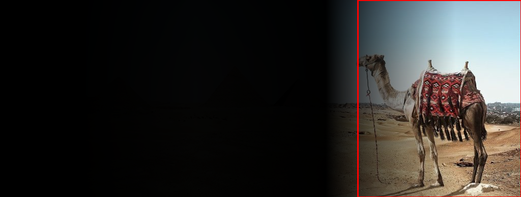
Visualization concerns:
from google.colab.patches import cv2_imshow
#
 Find the n x m score map for the predicted class
score_map = preds[0, predicted_class, :, :].cpu().numpy()
score_map = score_map[0]

# Resize score map to the original image size
score_map = cv2.resize(score_map, (original_image.shape[1], original_image.shape[0]))

# Binarize score map
_, score_map_for_contours = cv2.threshold(score_map, 0.25, 1, type=cv2.THRESH_BINARY)
score_map_for_contours = score_map_for_contours.astype(np.uint8).copy()

# Find the countour of the binary blob
contours, _ = cv2.findContours(score_map_for_contours, mode=cv2.RETR_EXTERNAL, method=cv2.CHAIN_APPROX_SIMPLE)

# Find bounding box around the object.
rect = cv2.boundingRect(contours[0])
# Apply score map as a mask to original image
score_map = score_map - np.min(score_map[:])
score_map = score_map / np.max(score_map[:])
score_map = cv2.cvtColor(score_map, cv2.COLOR_GRAY2BGR)
masked_image = (original_image * score_map).astype(np.uint8)

# Display bounding box
cv2.rectangle(masked_image, rect[:2], (rect[0] + rect[2], rect[1] + rect[3]), (0, 0, 255), 2)

# Display images
#cv2.imshow("Original Image", original_image)
#cv2.imshow("activations_and_bbox", masked_image)
cv2_imshow(original_image)
cv2_imshow(masked_image)
cv2.waitKey(0)
In Google collab, ipynb uses: from google.colab.patches import cv2_imshow
reference resources: https://www.learnopencv.com/cnn-receptive-field-computation-using-backprop/?ck_subscriber_id=503149816