Credit card fraud can be classified as an exception and can be detected using an automatic encoder implemented in Keras

I recently read an article called "using automatic encoder for anomaly detection", in which the generated data is tested, and I think it seems a good idea to apply the idea of using automatic encoder for anomaly detection to fraud detection in the real world.

I decided to use credit card fraud data from Kaggle: this data set contains credit card transaction information for European cardholders in September 2013.

This dataset shows transactions that occurred in two days, 492 of 284807 transactions were fraudulent data. Such data sets are quite unbalanced, in which positive (fraud) data accounts for 0.172% of all transaction data.

data mining

Although this is a very unbalanced data set, it is also a good example: to identify and verify exceptions or fraud.

First of all, we need to reduce the dimension of data set from 30 dimension to 3 dimension by principal component analysis, and draw the corresponding point graph. There are 32 columns in this dataset, the first column is time, 29 columns are unknown data, 1 column is transaction amount and the remaining 1 column is category. It should be noted that we will ignore the indicator of time, because it is not a more fixed indicator.

def show_pca_df(df):
	x = df[df.columns[1:30]].to_numpy()
	y = df[df.columns[30]].to_numpy()

	x = preprocessing.MinMaxScaler().fit_transform(x)
	pca = decomposition.PCA(n_components=3)
	pca_result = pca.fit_transform(x)
	print(pca.explained_variance_ratio_)

	pca_df = pd.DataFrame(data=pca_result, columns=['pc_1', 'pc_2', 'pc_3'])
	pca_df = pd.concat([pca_df, pd.DataFrame({'label': y})], axis=1)

	ax = Axes3D(plt.figure(figsize=(8, 8)))
	ax.scatter(xs=pca_df['pc_1'], ys=pca_df['pc_2'], zs=pca_df['pc_3'], c=pca_df['label'], s=25)
	ax.set_xlabel("pc_1")
	ax.set_ylabel("pc_2")
	ax.set_zlabel("pc_3")
	plt.show()

df = pd.read_csv('creditcard.csv')

show_pca_df(df)

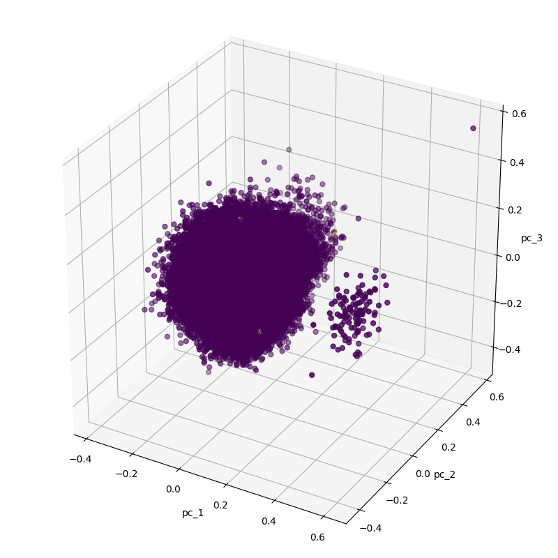
Looking at the above figure, you can see that there are two separate clusters. This seems to be a very simple task, but in fact, the fraud data is only yellow dots. If you look closely, in the larger cluster, we can see three yellow dots. As a result, we resampled normal data while retaining fraud data.

df_anomaly = df[df[df.columns[30]] > 0]
df_normal = df[df[df.columns[30]] == 0].sample(n=df_anomaly.size, random_state=1, axis='index')
df = pd.concat([ df_anomaly, df_normal])

show_pca_df(df)

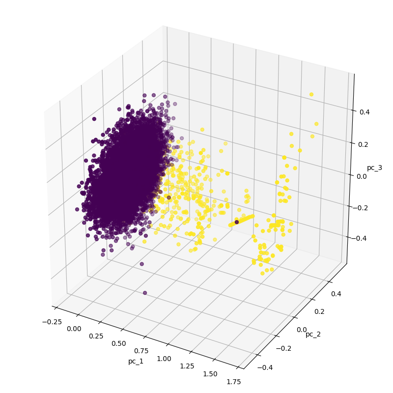
As can be seen from the above figure, the normal data is relatively centralized, similar to a disc, while the fraud data is relatively scattered. At this time, we will build an automatic encoder, which has a 3-layer encoder and a 2-layer decoder, as follows:

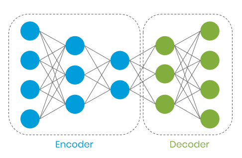
The automatic encoder encodes our data into a subspace and decodes it into corresponding features when normalizing the data. We hope that the automatic encoder can learn the features in the normalized conversion, and the input and output are similar in the application. In the case of exception, since it is fraudulent data, the input and output will be significantly different.

The advantage of this method is that it allows the use of unsupervised learning methods. After all, most of the data we usually use are normal transaction data. And the data label is usually difficult to obtain, and in some cases, it can not be used at all, for example, manual data labeling often has human cognitive bias and other problems. Thus, in the process of training the model, we only use the normal transaction data without labels.

Next, let's download the data and train the automatic encoder:

df = pd.read_csv('creditcard.csv')

x = df[df.columns[1:30]].to_numpy()
y = df[df.columns[30]].to_numpy()

# prepare data
df = pd.concat([pd.DataFrame(x), pd.DataFrame({'anomaly': y})], axis=1)
normal_events = df[df['anomaly'] == 0]
abnormal_events = df[df['anomaly'] == 1]

normal_events = normal_events.loc[:, normal_events.columns != 'anomaly']
abnormal_events = abnormal_events.loc[:, abnormal_events.columns != 'anomaly']

# scaling
scaler = preprocessing.MinMaxScaler()
scaler.fit(df.drop('anomaly', 1))

scaled_data = scaler.transform(normal_events)

# 80% percent of dataset is designated to training
train_data, test_data = model_selection.train_test_split(scaled_data, test_size=0.2)

n_features = x.shape[1]

# model
encoder = models.Sequential(name='encoder')
encoder.add(layer=layers.Dense(units=20, activation=activations.relu, input_shape=[n_features]))
encoder.add(layers.Dropout(0.1))
encoder.add(layer=layers.Dense(units=10, activation=activations.relu))
encoder.add(layer=layers.Dense(units=5, activation=activations.relu))

decoder = models.Sequential(name='decoder')
decoder.add(layer=layers.Dense(units=10, activation=activations.relu, input_shape=[5]))
decoder.add(layer=layers.Dense(units=20, activation=activations.relu))
decoder.add(layers.Dropout(0.1))
decoder.add(layer=layers.Dense(units=n_features, activation=activations.sigmoid))

autoencoder = models.Sequential([encoder, decoder])

autoencoder.compile(
	loss=losses.MSE,
	optimizer=optimizers.Adam(),
	metrics=[metrics.mean_squared_error])

# train model
es = EarlyStopping(monitor='val_loss', min_delta=0.00001, patience=20, restore_best_weights=True)
history = autoencoder.fit(x=train_data, y=train_data, epochs=100, verbose=1, validation_data=[test_data, test_data], callbacks=[es])
plt.plot(history.history['loss'])
plt.plot(history.history['val_loss'])
plt.title('Model Loss')
plt.ylabel('Loss')
plt.xlabel('Epoch')
plt.legend(['Train', 'Test'], loc='upper left')
plt.show()

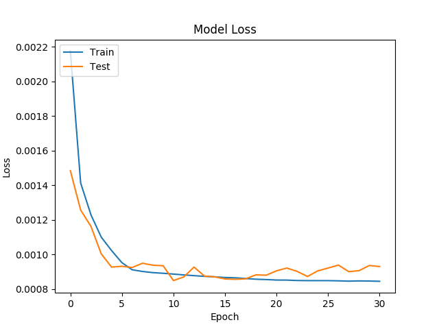
It can be seen from the following figure that the error of the model is about 8.5641e-04, while the minimum error is about 5.4856e-04.

Using this model, we can calculate the RMS error of normal trading, and also know how much threshold should be set when the RMS error value is 95%.

train_predicted_x = autoencoder.predict(x=train_data)
train_events_mse = losses.mean_squared_error(train_data, train_predicted_x)
cut_off = np.percentile(train_events_mse, 95)

The threshold value we set is 0.002. If the root mean square error is greater than 0.002, we will regard this transaction as an abnormal transaction, i.e. fraud. Let's select 100 fraud data and 100 normal data as samples, and the threshold can be plotted as follows:

plot_samples = 100
# normal event
real_x = test_data[:plot_samples].reshape(plot_samples, n_features)
predicted_x = autoencoder.predict(x=real_x)
normal_events_mse = losses.mean_squared_error(real_x, predicted_x)
normal_events_df = pd.DataFrame({
	'mse': normal_events_mse,
	'n': np.arange(0, plot_samples),
	'anomaly': np.zeros(plot_samples)})



# abnormal event
abnormal_x = scaler.transform(abnormal_events)[:plot_samples].reshape(plot_samples, n_features)
predicted_x = autoencoder.predict(x=abnormal_x)
abnormal_events_mse = losses.mean_squared_error(abnormal_x, predicted_x)
abnormal_events_df = pd.DataFrame({
	'mse': abnormal_events_mse,
	'n': np.arange(0, plot_samples),
	'anomaly': np.ones(plot_samples)})

mse_df = pd.concat([normal_events_df, abnormal_events_df])
plot = sns.lineplot(x=mse_df.n, y=mse_df.mse, hue=mse_df.anomaly)

line = lines.Line2D(
	xdata=np.arange(0, plot_samples),
	ydata=np.full(plot_samples, cut_off),
	color='#CC2B5E',
	linewidth=1.5,
	linestyle='dashed')

plot.add_artist(line)
plt.title('Threshlold: {threshold}'.format(threshold=cut_off))
plt.show()

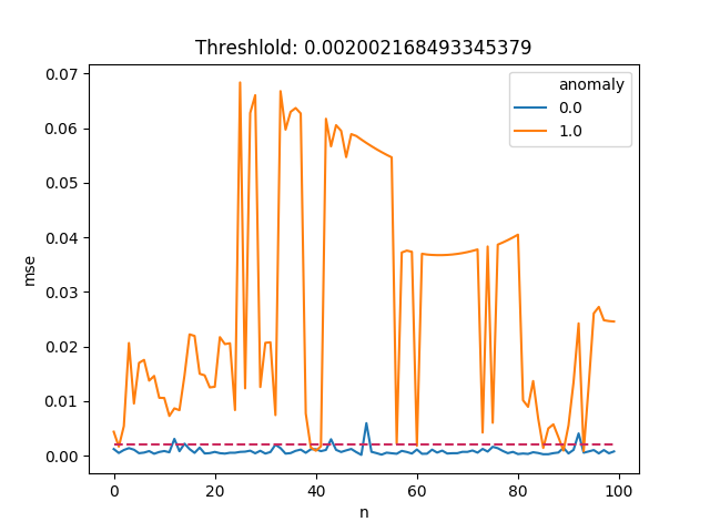
It can be seen from the above figure that most of the fraud data have higher root mean square error compared with the normal transaction data, so this method seems to be very effective for the identification of fraud data.

Although we have abandoned 5% of normal transactions, there are still fraudulent transactions below the threshold. This may be improved by using better feature extraction methods, because some fraud data and normal transaction data have very similar features. For example, for credit card fraud, if the transaction occurs in different countries, the more valuable characteristics are: the number of transactions in the previous hour, the previous day, and the previous week.

Next steps

1. Optimize the super parameters.

2. Use some data analysis methods to better understand the characteristics of data.

3.
Compare the above methods with other machine learning methods, such as support vector machine or k-means clustering and so on.

The complete code of this article can be obtained on Github.

https://github.com/bgokden/anomaly-detection-with-autoencoders

References

1. Andrea Dal Pozzolo, Olivier Caelen, Reid A. Johnson and Gianluca
Bontempi. Calibrating Probability with Undersampling for Unbalanced
Classification. In Symposium on Computational Intelligence and Data
Mining (CIDM), IEEE, 2015

2. Dal Pozzolo, Andrea; Caelen, Olivier; Le Borgne, Yann-Ael;
Waterschoot, Serge; Bontempi, Gianluca. Learned lessons in credit card
fraud detection from a practitioner perspective, Expert systems with
applications,41,10,4915–4928,2014, Pergamon

3. Dal Pozzolo, Andrea; Boracchi, Giacomo; Caelen, Olivier; Alippi,
Cesare; Bontempi, Gianluca. Credit card fraud detection: a realistic
modeling and a novel learning strategy, IEEE transactions on neural
networks and learning systems,29,8,3784–3797,2018,IEEE

4. Dal Pozzolo, Andrea Adaptive Machine learning for credit card fraud
detection ULB MLG PhD thesis (supervised by G. Bontempi)

5. Carcillo, Fabrizio; Dal Pozzolo, Andrea; Le Borgne, Yann-Aël;
Caelen, Olivier; Mazzer, Yannis; Bontempi, Gianluca. Scarff: a scalable
framework for streaming credit card fraud detection with Spark,
Information fusion,41, 182–194,2018,Elsevier

6. Carcillo, Fabrizio; Le Borgne, Yann-Aël; Caelen, Olivier; Bontempi,
Gianluca. Streaming active learning strategies for real-life credit card
fraud detection: assessment and visualization, International Journal of
Data Science and Analytics, 5,4,285–300,2018,Springer International
Publishing

7．Bertrand Lebichot, Yann-Aël Le Borgne, Liyun He, Frederic Oblé,
Gianluca Bontempi Deep-Learning Domain Adaptation Techniques for Credit
Cards Fraud Detection, INNSBDDL 2019: Recent Advances in Big Data and
Deep Learning, pp 78–88, 2019

8. Fabrizio Carcillo, Yann-Aël Le Borgne, Olivier Caelen, Frederic
Oblé, Gianluca Bontempi Combining Unsupervised and Supervised Learning
in Credit Card Fraud Detection Information Sciences, 2019

By Berk G ö kden

Deep hub translation team: Li AI