In the previous lesson, we talked about table method. In this lesson, we mainly used neural network method to solve the problem. Here, the teacher also talked about neural network thoroughly, which gave me a new understanding of neural network

This is the cliff problem of the last lesson: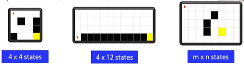

These palaces are countable, and can be installed with a Q form

However, in real life, there are many problems that are huge, even uncountable: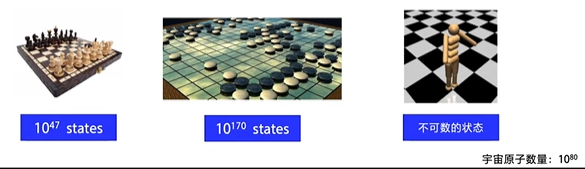

These States must not be loaded by the Q table. At this time, we need to use the approximation of the value function

Value function approximation

Value function is Q function. The function of Q table is to look up the table and output Q value according to the action of input state

Disadvantages of table method:

1. Tables can take up a lot of memory
2. When the table is very large, the efficiency of checking the table is low

In fact, we can use the Q function with parameters to approximate the Q table, such as polynomial function or neural network

Advantages of using value function approximation:

1. Only limited parameters need to be stored
2. State generalization, similar states can output the same

neural network

Neural network is actually like a huge function, which can convert the input x into the output y we want

If the input and output are vectors, then multiple inputs can be converted into multiple outputs

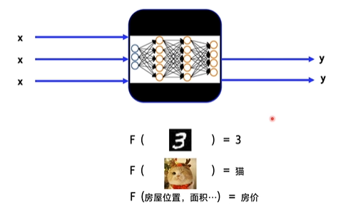
If you input a picture of the number 3, it will output 3; if you input a picture of the cat, it will output the cat classification; if you input the location and area of the house, it will output the predicted house price.

As long as you give it enough data, neural network can help you fit the continuous function you need

In fact, neural network is built up by one layer of functions. It can approximate any continuous function: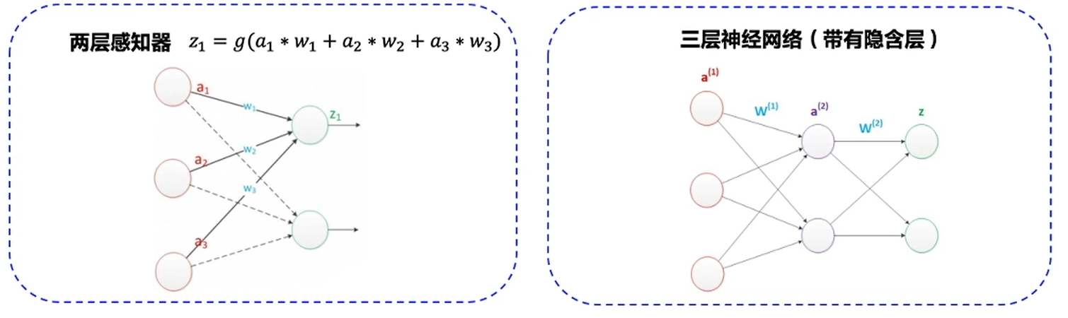


This is an example of using neural network to solve the 4 yuan equation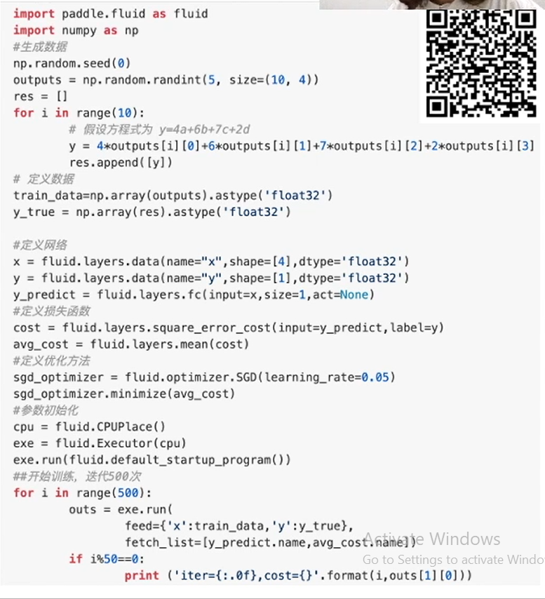

The above seemingly dense code, in fact, its process is not very complex: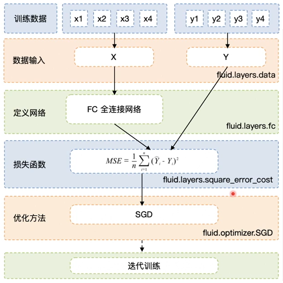

DQN: a classical algorithm for RL problem using neural network

DQN uses neural network to replace Q table approximately, but in essence, DQN is still a Q-learning algorithm with the same update mode.

The original Q-learning used a Q table: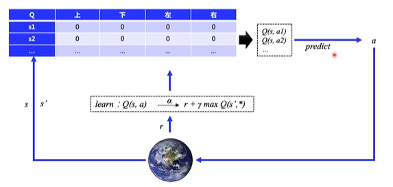

DQN's improvement is to replace Q table with neural network: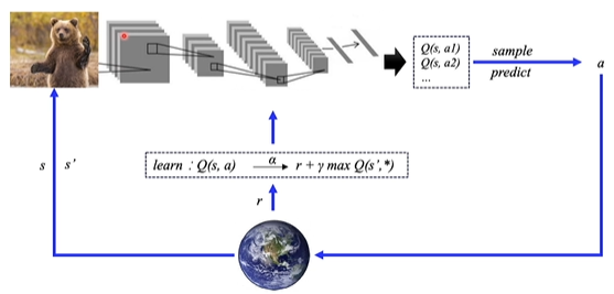

Input state and output action corresponding to all States

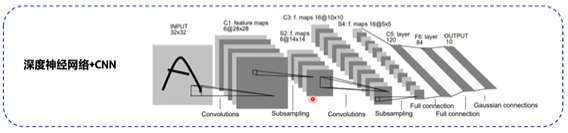
• If the state is a picture, the neural network can add a structure like CNN to extract features;
• If the state is a set of vectors, such as the state of a four-axis vehicle (height, rotation angle, speed, etc.), several full connection layers can be used for fitting

DQN ≈ Q-learning + neural network

Here is an analogy of how supervised learning is trained: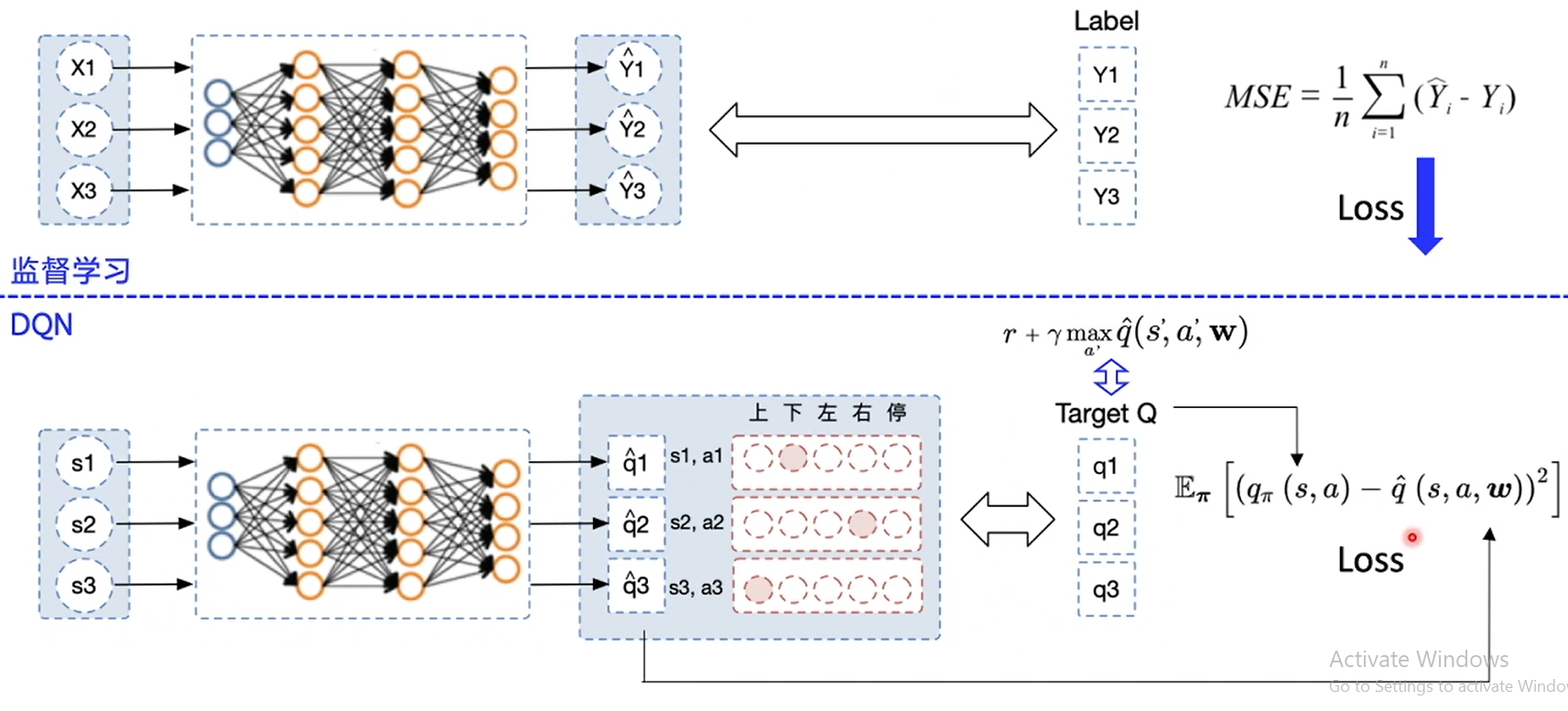

In supervised learning, after inputting x, the output prediction value y of the network should be close to the real value label of Y as much as possible. At this time, we can directly find their mean square deviation, that is, loss, and send it into the optimization function, then we can automatically update and optimize the network

The training process of DQN is also very similar. It inputs a batch of States and outputs the corresponding Q value. The Q value is actually a vector. Assuming that the action dimension is 5, each action will correspond to a Q value. According to the actual action, the corresponding Q value should be taken. It is also necessary to make the Q value come close to my target value Target Q. to update the neural network, the same is true, The mean square deviation is calculated and then brought into the optimization function, so that the network parameters can be updated automatically

DQN algorithm analysis

On the basis of Q-learning, DQN proposes two techniques to make the update iteration of q-network more stable:

• Experience Replay: it mainly solves the problems of sample relevance and utilization efficiency. A pool of experiences is used to store multiple experiences s,a,r,s', from which a batch of data is randomly selected for training.
• Fixed-Q-Target: it mainly solves the problem of unstable algorithm training. Copy a Target Q network with the same structure as the original Q network to calculate the Q target value.

Experience playback: take full advantage of off policy

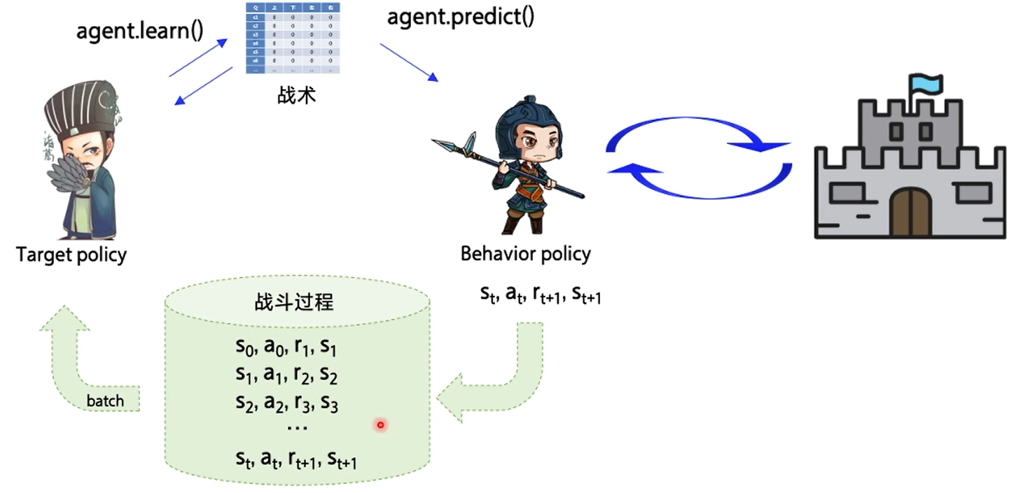
On the basis of the original, a buffer is added to store the experience of behavioral strategies. When the experience reaches a certain amount, the target strategy scrambles the time sequence of the experience, takes it out according to the amount of a batch, and then updates the Q table

The benefits of doing so are:

1. Disarrange sample relevance
2. Improve sample utilization

Its implementation code is as follows:

import random
import collections
import numpy as np


class ReplayMemory(object):
    def __init__(self, max_size):
        self.buffer = collections.deque(maxlen=max_size) # queue

    # Add an experience to the experience pool
    def append(self, exp):
        self.buffer.append(exp)

    # Select N experiences from the experience pool
    def sample(self, batch_size):
        mini_batch = random.sample(self.buffer, batch_size)
        obs_batch, action_batch, reward_batch, next_obs_batch, done_batch = [], [], [], [], []

        for experience in mini_batch:
            s, a, r, s_p, done = experience
            obs_batch.append(s)
            action_batch.append(a)
            reward_batch.append(r)
            next_obs_batch.append(s_p)
            done_batch.append(done)

		# Split into 5 arrays
        return np.array(obs_batch).astype('float32'), \
            np.array(action_batch).astype('float32'), np.array(reward_batch).astype('float32'),\
            np.array(next_obs_batch).astype('float32'), np.array(done_batch).astype('float32')

    def __len__(self):
        return len(self.buffer)

Fixed Q target

Fixed Q target can solve the problem of unstable algorithm update

Here is also a comparison of supervised learning. After inputting x, it outputs the predicted value y, so that the predicted value is the real value after all, which is actually stable in supervised learning: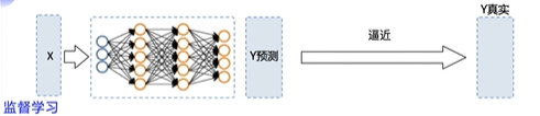
The predicted value of DQN output is also close to Q_target's: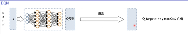

But the Q here actually has to go through the network, which leads to the constant change of the Q, which is like taking a moving rabbit as a target when practicing archery: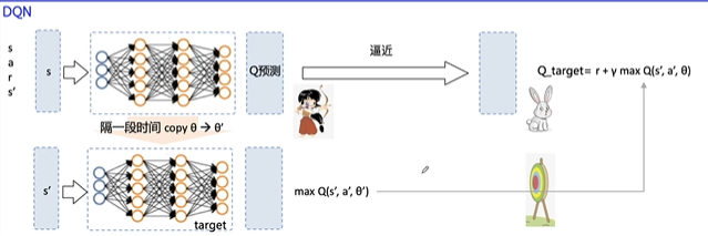

What the fixed Q target does is to keep the Q unchanged for a period of time, and then copy the parameter for a period of time

The following is the flow chart of DQN algorithm: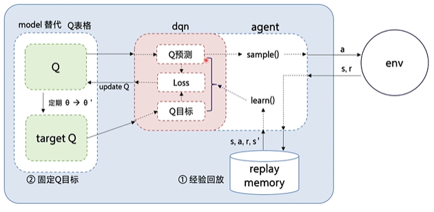

DQN implemented in PARL separates the nested parts: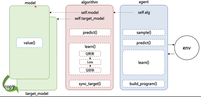

The model part is used to define the network structure with neural network, which can be Q network or policy network, etc

Here is the framework of the PARL: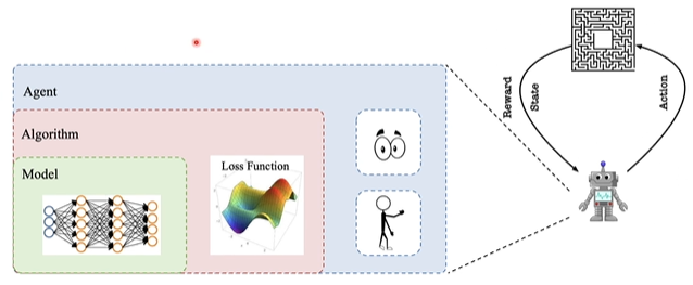

Code analysis of PARL DQN

Agent transmits the generated data to algorithm, which calculates the Loss according to the model structure, and optimizes it continuously by SGD or other optimizers. The PARL architecture can be easily used in various deep reinforcement learning problems.

model

Model is used to define the forward network. Users can customize their own network structure freely.

class Model(parl.Model):
    def __init__(self, act_dim):
        hid1_size = 128
        hid2_size = 128
        # Layer 3 fully connected network
        self.fc1 = layers.fc(size=hid1_size, act='relu')
        self.fc2 = layers.fc(size=hid2_size, act='relu')
        self.fc3 = layers.fc(size=act_dim, act=None)

    def value(self, obs):
        # Define network
        # Input state, output Q corresponding to all action s, [Q(s,a1), Q(s,a2), Q(s,a3)...]
        h1 = self.fc1(obs)
        h2 = self.fc2(h1)
        Q = self.fc3(h2)
        return Q

This is a very simple fully connected network with only three layers. The activation function of the first two layers is relu

algorithm

Algorithm defines a specific algorithm to update the forward network (Model), that is, to update the Model by defining the loss function, and algorithm related calculations are put in algorithm.

Here we need to input the model just defined

# from parl.algorithms import DQN # You can also import DQN algorithm directly from the parl Library

class DQN(parl.Algorithm):
    def __init__(self, model, act_dim=None, gamma=None, lr=None):
        """ DQN algorithm
        
        Args:
            model (parl.Model): definition Q Forward network structure of function
            act_dim (int): action There are several dimensions of space action
            gamma (float): reward Attenuation factor of
            lr (float): learning rate Learning rate.
        """
        self.model = model
        self.target_model = copy.deepcopy(model)

        assert isinstance(act_dim, int)
        assert isinstance(gamma, float)
        assert isinstance(lr, float)
        self.act_dim = act_dim
        self.gamma = gamma
        self.lr = lr

Use deep copy () to copy the model quickly

After defining DQN, you need to implement sync_target() method:

def sync_target(self):
    """ hold self.model Model parameter values of are synchronized to self.target_model
    """
    self.model.sync_weights_to(self.target_model)

The api can be called directly here, and the PARL has been implemented by users

The purpose of this method is to periodically_ The parameters of the model are synchronized to the model

Similarly, implementing the predict() method is simple:

def predict(self, obs):
    """ use self.model Of value Network to get [Q(s,a1),Q(s,a2),...]
    """
    return self.model.value(obs)

Just return the output value of model directly

Next, the core method is the learn() method:

def learn(self, obs, action, reward, next_obs, terminal):
    """ use DQN Algorithm update self.model Of value network
    """
    # From target_ Get the value of max Q 'in the model, which is used to calculate target Qu
    next_pred_value = self.target_model.value(next_obs)
    best_v = layers.reduce_max(next_pred_value, dim=1)
    best_v.stop_gradient = True  # Prevent gradient transfer
    terminal = layers.cast(terminal, dtype='float32')
    target = reward + (1.0 - terminal) * self.gamma * best_v

    pred_value = self.model.value(obs)  # Get Q forecast
    # Transfer action to onehot vector, for example: 3 = > [0,0,0,1,0]
    action_onehot = layers.one_hot(action, self.act_dim)
    action_onehot = layers.cast(action_onehot, dtype='float32')
    # The next line is to multiply each element to get the Q(s,a) corresponding to action
    # For example: pred_value = [[2.3, 5.7, 1.2, 3.9, 1.4]], action_onehot = [[0,0,0,1,0]]
    #  ==> pred_action_value = [[3.9]]
    pred_action_value = layers.reduce_sum(
        layers.elementwise_mul(action_onehot, pred_value), dim=1)

    # Calculate Q(s,a) and target_ The mean square deviation of Q gives loss
    cost = layers.square_error_cost(pred_action_value, target)
    cost = layers.reduce_mean(cost)
    optimizer = fluid.optimizer.Adam(learning_rate=self.lr)  # Using the Adam optimizer
    optimizer.minimize(cost)
    return cost

Although it is the most core part, it is not difficult. It can be divided into three parts to understand:
In the first block, calculate the target value; in the second block, calculate the predicted value; in the third block, get the loss

It used to use if condition judgment when calculating target-Q, but here is a very clever way:

terminal = layers.cast(terminal, dtype='float32')
target = reward + (1.0 - terminal) * self.gamma * best_v

The terminal entered here is actually the original data used to determine whether the last data is done

The clever thing is that you can convert this done to a floating-point number, that is, True is 1, False is 0

Then subtract it from 1, and when terminal is True, 1 - 1 = 0, that part will be eliminated:

target = reward

When terminal is False, because 1 - 0 = 1, it does not affect

agent

Agent is responsible for the interaction between Algorithm and environment. In the interaction process, the generated data is provided to Algorithm to update the model. The preprocessing process of data is also generally defined here.

def learn(self, obs, act, reward, next_obs, terminal):
    # Synchronize model and target every 200 training steps_ Parameters of model
    if self.global_step % self.update_target_steps == 0:
        self.alg.sync_target()
    self.global_step += 1

    act = np.expand_dims(act, -1)
    feed = {
        'obs': obs.astype('float32'),
        'act': act.astype('int32'),
        'reward': reward,
        'next_obs': next_obs.astype('float32'),
        'terminal': terminal
    }
    cost = self.fluid_executor.run(self.learn_program, feed=feed, fetch_list=[self.cost])[0]  # Training a network
    return cost

A feed stores input_ List stores build_ Output of the program () method

When calculating loss, run() will be executed once, i.e. update the network once

In build_ The shape of each variable is defined in the program () method

def build_program(self):
    self.pred_program = fluid.Program()
    self.learn_program = fluid.Program()

    with fluid.program_guard(self.pred_program):  # Build calculation chart to predict actions and define input and output variables
        obs = layers.data(
            name='obs', shape=[self.obs_dim], dtype='float32')
        self.value = self.alg.predict(obs)

    with fluid.program_guard(self.learn_program):  # Build calculation chart to update Q network and define input and output variables
        obs = layers.data(
            name='obs', shape=[self.obs_dim], dtype='float32')
        action = layers.data(name='act', shape=[1], dtype='int32')
        reward = layers.data(name='reward', shape=[], dtype='float32')
        next_obs = layers.data(
            name='next_obs', shape=[self.obs_dim], dtype='float32')
        terminal = layers.data(name='terminal', shape=[], dtype='bool')
        self.cost = self.alg.learn(obs, action, reward, next_obs, terminal)

The last two methods are:

def sample(self, obs):
    sample = np.random.rand()  # Generate decimal between 0 and 1
    if sample < self.e_greed:
        act = np.random.randint(self.act_dim)  # Exploration: every action has a probability to be selected
    else:
        act = self.predict(obs)  # Choose the best action
    self.e_greed = max(
        0.01, self.e_greed - self.e_greed_decrement)  # As the training gradually converges, the degree of exploration gradually decreases
    return act

def predict(self, obs):  # Choose the best action
    obs = np.expand_dims(obs, axis=0)
    pred_Q = self.fluid_executor.run(
        self.pred_program,
        feed={'obs': obs.astype('float32')},
        fetch_list=[self.value])[0]
    pred_Q = np.squeeze(pred_Q, axis=0)
    act = np.argmax(pred_Q)  # Select Q maximum subscript, i.e. corresponding action
    return act

In general, there are three classes and eight methods:

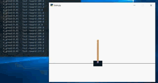
DQN training show CartPole

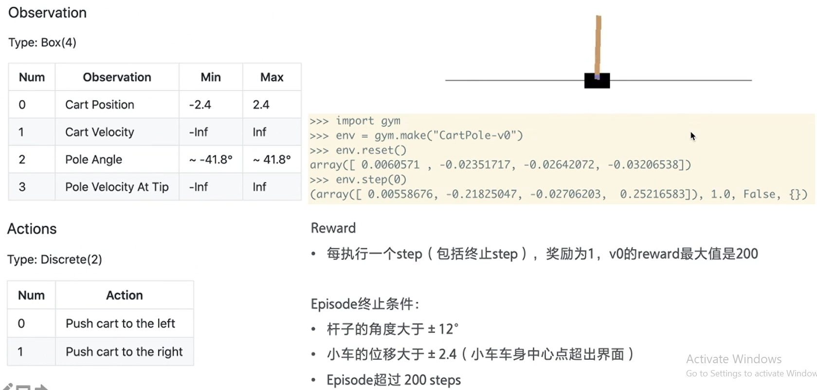
The code of this part is in parson3: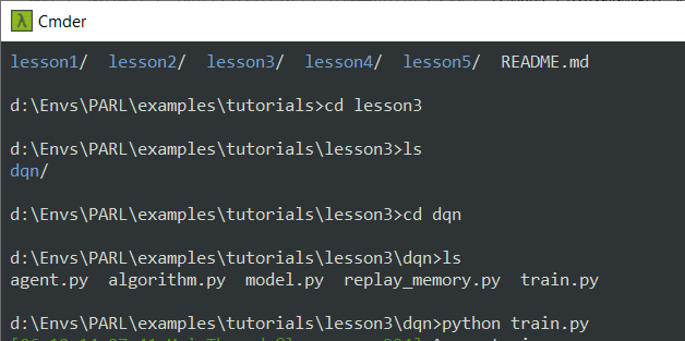

Run the following: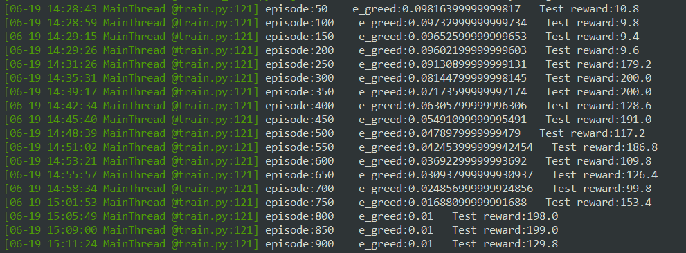

It can be seen that its score is good or bad. Even taking the trained model for testing, it may be better or worse than the original

In fact, like people, it is inevitable to fail. Every time the environment is random, so every run may be different. The following is a dynamic diagram

At the beginning of the training, it will end because the inclination is too large: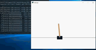

When there are more than one thousand episode s, the pole basically master the rules of the game, but it is easy to slide out: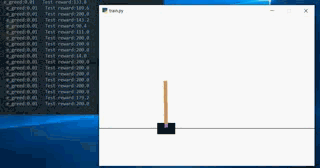

When training to about 2000 episode s, they basically don't slide out: