Deep learning target tracking
1. Essence: get characteristic map, output classification and location by convolution neural network.
2. Classification of target tracking:
① Single class multitarget tracking: MTCNN, Retinaface
② Multi class and multi-target tracking: RCNN, spp net, fast RCNN / fast RCNN, SSD
(1) RCNN:
The search box (forced scaling) is obtained by clustering, and the features are extracted by convolution, and then classified by SVM.
Slow speed, low accuracy.
(2) SPP-Net:
Space pyramid pooling is mainly used to scale different size boxes. The scaled size can enter FC layer for output.
(4)Fast-RCNN:
Steps: CNN convolution, candidate box, ROIPooling layer, FC output.
Candidate boxes are obtained by selective search. It is very time-consuming to find all candidate boxes.
The purpose of the ROIPooling layer is to resize the candidate boxes to a uniform size.
(5)Faster-RCNN
Replace ROI in FastRCNN with RPN network.
(6) Summary:
It can be seen that most of the problems and improvements in multi-target tracking focus on the selection of candidate boxes. After yoloV2, the selection of candidate boxes introduces the anchor mechanism.
yolo (you only look once)
1. yoloV1:
(1) Step:
The first step is to divide the original image into S * S cells. (7 * 7) each lattice has its own confidence degree, through which we can judge whether there is a target in the lattice and classify it. If the grid has a target, go to step 2.
In the second step, each grid can get two suggestion boxes according to its center point, (two boxes with the center point as the origin are set in advance / the essence is the anchor box), that is, the center point is fixed, and the suggestion box and the actual box are offset.
(2) Disadvantage: a grid can only determine one target. (in the actual picture, a grid may contain more than one target / kind of information); and when there are small objects or large objects, it is difficult to predict.
(3) Input / output: input 448 * 448 * 3 pictures, output 7 * 7 * (5 * 2 + 20). That is, 49 grids, 2 anchor boxes per grid (confidence + coordinate position), 20 categories.
(4) Loss function: confidence loss + coordinate loss + category loss.
2. yoloV2
(1) Backbone network: darknet19
The whole network is convolution, so it can be multi-dimensional input.
In practice, the anchor mechanism is used to change the input to 416 * 416.
The output layer is changed to the output we need through an output layer.
(2) Anchor: according to the real frame position of the data set, five anchor frames are obtained by clustering, which are used as the suggestion boxes of each grid.
(3) I / O: pictures with input of 416 * 416 * 3 and output of 13 * 13 * 5 * (5 + 20). That is to say, the picture is divided into 13 * 13 grids, each grid has 5 anchor boxes, and each anchor box has a category label (20 categories).
(4) Offset: labels are converted to offset for operation.
Position of prediction point center: cx, cy - > offcx offcy
(for example, the position of the actual center point, cx = 13 * (offcx + index), the offset of the center point of the offcx from the upper left corner of the lattice, and the index of the index lattice)
That is to say, the output of neural network, each grid has five anchor centers, each center can get the actual position through the grid size.
Width and height of prediction box: bw BH - > offw offh
The width height is the ratio of the prediction box to the actual box, and the log operation is carried out (making the offset near 0 to prevent gradient dispersion).
(4) Loss function: confidence loss + coordinate loss + category loss. Different from yoloV1, each anchor here has its own category label.
3. yolo9000
Build tree structure for classification. Didn't understand in detail. You can see this.
4. yoloV3
(1) Backbone network: darknet53
In the backbone network structure, the feature map obtained from the last three undersampling will be used as the prediction.
In short, it's a feature map of different sizes. Each grid represents a different feeling field. The receptive field in the lower layer is larger than that in the upper layer, which contains more semantic information. Therefore, the superposition of the upper layer and the lower layer can retain more semantic information. Finally, we enter the prediction layer to get the output. Because the last three subsamples predict respectively, each lattice has three anchor frames (13 * 13, 26 * 26, 52 * 52 size of the feature map). According to the size of the feature map, the predicted objects are different in size.
You can read this in detail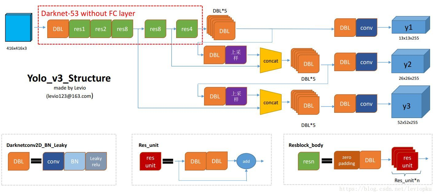
I have written the network structure of yoloV3 with pytorch. Here is the main network part. Some network blocks have to be written by myself. For example, the convolutional layer is DBL (convolution, batchnorm, relu activation), down sampling block, up sampling block, residual network
The third subsampling is used as the prediction output, and the last second subsampling output and the third subsampling feature map (after the upper sampling) are superposed; similarly, the first subsampling and the second and third superposing feature map are superposed.
class yoloV3_net(nn.Module):
    def __init__(self):
        super(yoloV3_net,self).__init__()

        self.trunk_52 = nn.Sequential(
            ConvolutionalLayer(3,32,3,1,1),
            DownsamplingLayer(32,64),
            ResidualLayer(64),
            DownsamplingLayer(64,128),
            ResidualLayer(128),
            ResidualLayer(128),
            DownsamplingLayer(128,256),
            ResidualLayer(256),
            ResidualLayer(256),
            ResidualLayer(256),
            ResidualLayer(256),
            ResidualLayer(256),
            ResidualLayer(256),
            ResidualLayer(256),
            ResidualLayer(256),
        )

        self.trunk_26 = nn.Sequential(
            DownsamplingLayer(256,512),
            ResidualLayer(512),
            ResidualLayer(512),
            ResidualLayer(512),
            ResidualLayer(512),
            ResidualLayer(512),
            ResidualLayer(512),
            ResidualLayer(512),
            ResidualLayer(512),
        )

        self.trunk_13 = nn.Sequential(
            DownsamplingLayer(512,1024),
            ResidualLayer(1024),
            ResidualLayer(1024),
            ResidualLayer(1024),
            ResidualLayer(1024),
        )

        self.convset_13 = nn.Sequential(
            ConvolutionalSet(1024,512)
        )
        self.detetion_13 = nn.Sequential(
            ConvolutionalLayer(512,1024,3,1,1),
            nn.Conv2d(1024,3*(5+5),1,1,0)
        )

        self.up_26 = nn.Sequential(
            ConvolutionalLayer(512,256,1,1,0),
            UpsampleLayer()
        )
        self.convset_26 = nn.Sequential(
            ConvolutionalSet(768,256)
        )
        self.detetion_26 = nn.Sequential(
            ConvolutionalLayer(256, 512, 3, 1, 1),
            nn.Conv2d(512, 3*(5+5), 1, 1, 0)
        )

        self.up_52 = nn.Sequential(
            ConvolutionalLayer(256, 128, 1, 1, 0),
            UpsampleLayer()
        )
        self.convset_52 = nn.Sequential(
            ConvolutionalSet(384, 128)
        )
        self.detetion_52 = nn.Sequential(
            ConvolutionalLayer(128, 256, 3, 1, 1),
            nn.Conv2d(256, 3*(5+5), 1, 1, 0)
        )

    def forward(self,x):
        # Convolution layer to get characteristic graphs of different sizes
        h_52 = self.trunk_52(x)
        h_26 = self.trunk_26(h_52)
        h_13 = self.trunk_13(h_26)
        # 13
        convset_out_13 = self.convset_13(h_13)
        detetion_out_13 = self.detetion_13(convset_out_13)
        up_13to26 = self.up_26(convset_out_13)
        # 26
        route_out_13and26 = torch.cat((up_13to26,h_26),dim=1)
        convset_out_26 = self.convset_26(route_out_13and26)
        detetion_out_26 = self.detetion_26(convset_out_26)
        up_26to52 = self.up_52(convset_out_26)
        # 52
        route_out_26and52 = torch.cat((up_26to52, h_52), dim=1)
        convset_out_52 = self.convset_52(route_out_26and52)
        detetion_out_52 = self.detetion_52(convset_out_52)
        return detetion_out_13,detetion_out_26,detetion_out_52
(2) Data: coco data set - because the computer can't carry yolo for training, when learning, I choose more than 100 pictures and 5 categories for training. (get the over fitting version - that is, the training set is the test set)
① First scale the data to 416 * 416. Equal scale, the missing part is filled with black.
import cv2
import os
def cv2_letterbox_image(image, expected_size):
    ih, iw = image.shape[0:2]
    ew, eh = expected_size,expected_size
    scale = min(eh / ih, ew / iw) # Scale the maximum edge to 416
    nh = int(ih * scale)
    nw = int(iw * scale)
    image = cv2.resize(image, (nw, nh), interpolation=cv2.INTER_CUBIC) # Scale equally so that one side 416
    top = (eh - nh) // 2 # Height of upper part fill
    bottom = eh - nh - top  # Height of lower part fill
    left = (ew - nw) // 2 # Left part fill distance
    right = ew - nw - left # Distance of right part fill
    # Boundary fill
    new_img = cv2.copyMakeBorder(image, top, bottom, left, right, cv2.BORDER_CONSTANT)
    return new_img

if __name__ == '__main__':
    dir_root = "D:/AIstudyCode/data/yolo_data"
    save_dir = "data/"
    count = 0
    for path in os.listdir(dir_root):
        print(path)
        img = cv2.imread(f"D:/AIstudyCode/data/yolo_data/{path}")
        print(img.shape)
        new_img = cv2_letterbox_image(img,416)
        print(new_img.shape)
        cv2.imwrite(f"{save_dir}images/{count}.jpg",new_img)
        count += 1
        cv2.imshow("1",new_img)
        cv2.waitKey(5)
② Then the wizard annotation assistant is used to annotate, get the xml tags, and analyze them. Get the tag file txt, (easy to do dataset)
Format: file name path first anchor: Category c (box information) second anchor: Category c (box information)
③ dataset: parse the label and picture, and calculate the offset.
class MyDataset(Dataset):
    def __init__(self):
        with open(LABEL_FILE_PATH) as f:
            self.dataset = f.readlines() # Read label text line by line
            # img_path category 1 anchor box 4 category 1 anchor box 4 category 1 anchor box 1 anchor box 4
    def __len__(self):
        return len(self.dataset) # Each row represents as many rows of data as there are

    def __getitem__(self, index):
        labels = {} # Label dictionary picture path: Category
        line = self.dataset[index] # index
        strs = line.split() # Divide each line by space
        #_img_data = Image.open(os.path.join(IMG_BASE_DIR,strs[0])) # Path dir+path
        _img_data = Image.open(os.path.join(strs[0]))

        img_data = transfroms(_img_data) # Data preprocessing

        # Convert the category and confidence after read label from character format to floating-point type and save with list
        #_boxes = np.array(float(x) for x in strs[1:])
        _boxes = np.array(list(map(float,strs[1:])))

        # For example, three box es are 1 * 15 (Category 1 x1 y1 x2 y2...) : convert to 1 * 3 * 5
        boxes = np.split(_boxes, len(_boxes) // 5) # Separate the anchor

        # ANCHORS_GROUP feature size (13, 26, 52): size of three anchor s (w, h)
        for feature_size, anchors in cfg.ANCHORS_GROUP.items():
            # F*F *3*(5+c) each lattice has three anchor box c classifications: confidence degree 1+box position 4 + category number c
            # Initialization label storage dictionary is key: list / and table initialization is zero
            labels[feature_size] = np.zeros(shape=(feature_size,feature_size,3,5+cfg.CLASS_NUM))
            for box in boxes:
                cls, cx, cy, w, h = box # Get the real box in the label text

                # modf takes out the decimal part and the integer part respectively (the position of the actual box is equal to the feature size * (index + offset))
                cx_offset, cx_index = math.modf(cx * feature_size / cfg.IMG_WIDTH)
                cy_offset, cy_index = math.modf(cy * feature_size / cfg.IMG_WIDTH)
                # Take out the anchor size information which is defined in advance under different feature sizes
                for i, anchor in enumerate(anchors):
                    # Area under current anchor size
                    anchor_area = cfg.ANCHORS_GROUP_AREA[feature_size][i]
                    # The ratio of pw ph actual frame and anchor is taken as logarithm again: obtained by network training_ pw,_ PH - > through exp(_pw)*anchor_w / exp(_ph)*anchor_h to get the real frame
                    p_w, p_h = w / anchor[0], h / anchor[1]
                    _p_w, _p_h = np.log(p_w),np.log(p_h)
                    #print(_p_h,_p_w)
                    #Area of actual frame
                    p_area = w * h
                    # iou takes the minimum box / maximum box: in order to make iou (acting as confidence) less than 1 and greater than 0, it is biased to 1
                    iou = min(p_area,anchor_area) / max(p_area, anchor_area)
                    # Amplitude the label storage dictionary
                    # Offset of confidence center x y offset of width and height (relative to anchor) onehot category
                    labels[feature_size][int(cy_index), int(cx_index), i] = np.array(
                        [iou,cx_offset,cy_offset,_p_w,_p_h,*one_hot(cfg.CLASS_NUM,int(cls))])
                    #print(cx_offset)
                    #print(feature_size,cy_index,cx_index,i,"________",labels[feature_size][int(cy_index), int(cx_index), i])
                    #print(img_data)
        return labels[13], labels[26], labels[52], img_data
④ Network construction. (front network structure)
⑤ Loss design: confidence loss + coordinate loss + category loss.
# loss
def loss_fn(output, target, alpha):

    # torch.nn.BCELoss() must be activated with sigmoid
    conf_loss_fn = torch.nn.BCEWithLogitsLoss() # Binary cross entropy - > confidence with sigmoid+BCE

    crood_loss_fn = torch.nn.MSELoss() # Square difference - > box position
    cls_loss_fn = torch.nn.CrossEntropyLoss() # Cross entropy - > category
    # NLLLOSS log+softmax

    # N C H W -> N H W C
    output = output.permute(0, 2, 3, 1)
    # N C H W -> N H W 3 15
    output = output.reshape(output.size(0), output.size(1), output.size(2), 3, -1)
    output = output.cpu().double()
    mask_obj = target[..., 0] > 0
    output_obj = output[mask_obj]
    target_obj = target[mask_obj]

    loss_obj_conf = conf_loss_fn(output_obj[:,0], target_obj[:,0]) # Loss of confidence
    loss_obj_crood = crood_loss_fn(output_obj[:,1:5],target_obj[:,1:5]) # box loss
    # The loss function of cross entropy is the first predicted label, and the second parameter of onehot is the real label
    label_tags = torch.argmax(target_obj[:,5:], dim=1)
    #print(output_obj[:, 5:].shape, label_tags.shape)
    loss_obj_cls = cls_loss_fn(output_obj[:, 5:], label_tags) # Category loss

    loss_obj = loss_obj_cls + loss_obj_conf + loss_obj_crood # Total loss

    mask_noobj = target[..., 0] == 0 # When the data with iou 0 is trained in the anchor, the confidence level of the negative sample with confidence 0 only needs to be trained and the confidence level of the real tag
    output_noobj = output[mask_noobj]
    target_noobj = target[mask_noobj]
    loss_noobj = conf_loss_fn(output_noobj[:,0], target_noobj[:, 0])
    # Add by weight (the proportion of weight can be set according to the proportion of positive and negative samples in the dataset)
    loss = alpha * loss_obj + (1 - alpha) * loss_noobj

    return loss
⑥ Training:
if __name__ == '__main__':

    save_path = "data/checkpoints/myyolo.pt" #Where weights are saved
    myDataset = dataset.MyDataset()
    train_loader = DataLoader(myDataset, batch_size=2, shuffle=True)

    device = torch.device("cuda" if torch.cuda.is_available() else "cpu") #cuda or not
    net = yoloV3_net().to(device)

    if os.path.exists(save_path):
        net.load_state_dict(torch.load(save_path)) #Load weight
    else:
        print("NO Param!")

    net.train()
    opt = torch.optim.Adam(net.parameters())

    epoch = 0
    while(True):
        sum_loss = 0.
        for target_13, target_26, target_52, img_data in train_loader:
            img_data = img_data.to(device)
            output_13, output_26, output_52 = net(img_data)

            loss_13 = loss_fn(output_13, target_13, 0.5)
            loss_26 = loss_fn(output_26, target_26, 0.5)
            loss_52 = loss_fn(output_52, target_52, 0.5)
            loss = loss_13 + loss_26 + loss_52

            opt.zero_grad()
            loss.backward()
            opt.step()
            sum_loss += loss
            print("loss:",loss.item())
        avg_loss = sum_loss / len(train_loader)
        print("epoch:",epoch,"avg_loss:",avg_loss)
        if epoch % 10 == 0:
            torch.save(net.state_dict(),save_path)
            print('save{}'.format(epoch))

        epoch += 1
⑦ Detection part: zoom the image to 416 * 416 and enter the network to get the output.
The offset of the output is back calculated, and then filtered by iou and nms. The operation here is similar to that of MTCNN before.
class Detector(torch.nn.Module):
    def __init__(self, save_path):
        super(Detector, self).__init__()

        self.net = yoloV3_net().to(device) # Load network
        self.net.load_state_dict(torch.load(save_path)) # Load weight
        self.net.eval() # Mark here is the test

    def forward(self, input, thresh, anchors):
        # Input 416 * 416, output the data of each cell under different sizes F*F*3 * (5+c)
        output_13, output_26, output_52 = self.net(input)

        #print(output_13.shape)
        # Filtering boxes based on confidence returns index position and filtered boxes information
        idxs_13, vecs_13 = self._filter(output_13.to(_device), thresh)
        # Reverse the position of box in the original picture
        boxes_13 = self._parse(idxs_13, vecs_13, 32, anchors[13])
        idxs_26, vecs_26 = self._filter(output_26.to(_device), thresh)
        boxes_26 = self._parse(idxs_26, vecs_26, 16, anchors[26])
        idxs_52, vecs_52 = self._filter(output_52.to(_device), thresh)
        boxes_52 = self._parse(idxs_52, vecs_52, 8, anchors[52])
        # Return the final box information
        # print(boxes_13.shape)
        # print(boxes_26.shape)
        # print(boxes_52.shape)
        return torch.cat([boxes_13, boxes_26, boxes_52], dim=0)

    def _filter(self, output, thresh):
        output = output.permute(0,2,3,1) # N 3*(5+C) F F -> N F F 3*(5+C)
        output = output.reshape(output.size(0), output.size(1), output.size(2), 3, -1) # N F F 3*(5+C) -> N F F 3 5+C
        #print("1", output[:, 0])
        torch.sigmoid_(output[..., 0])
        #print("2",output[:, 0])

        mask = output[..., 0]>thresh # 5+C = confidence + cx cy w h the 0 th place is confidence
        #print(output[:, 0])
        idxs = mask.nonzero() # Get filtered location index
        #print("idxs",idxs.shape)
        vecs = output[mask] # Get the filtered boxes information
        return idxs, vecs

    def _parse(self, idxs, vecs, t, anchors):
        anchors = torch.Tensor(anchors)
        a = idxs[:,3] # Three anchor boxes
        confidence = vecs[:, 0]
        _classify = vecs[:, 5:]
        if len(_classify) == 0:
            classify = torch.Tensor([])
        else:
            classify = torch.argmax(_classify, dim=1).float() # One hot - > category

        # Inverse process
        cy = (idxs[:, 1].float() + vecs[:, 2]) * t
        cx = (idxs[:, 2].float() + vecs[:, 1]) * t
        w = anchors[a, 0] * torch.exp(vecs[:, 3])
        h = anchors[a, 1] * torch.exp(vecs[:, 4])
        x1 = cx - w / 2
        y1 = cy - h / 2
        x2 = x1 + w
        y2 = y1 + h
        out = torch.stack([confidence, x1, y1, x2, y2, classify],dim=1)
        return out