Thoughts and summary of Xiamen International Bank's "digital creation financial Cup" competition

Note: This is the first time to participate in the competition, the results are not ideal, experts do not spray...

1, Interpretation of competition questions

1. Tasks

2. Data

3. Scoring criteria

4. Solution to task

By analyzing the data labels, we can know that this is an unbalanced sample classification problem. For this kind of problem, we can deal with the task from the following methods:
(1) Build a classification model, deal with unbalanced data, and then classify
(2) Turn classification problem into outlier detection problem

2, Code details

1. Data processing

1.1 data exploration

1.1.1 analysis of data labels

(1) Import related packages and read data

import pandas as pd
import numpy as np
import matplotlib.pyplot as plt
import warnings  
warnings.filterwarnings('ignore')  #Ignore warnings
%matplotlib inline
pd.set_option('display.max_columns',None)  #Show all features
import time,datetime

test_df=pd.read_csv(r'C:\Users\Chen\Data mining competition\"Digital financial Cup" of Xiamen International Bank\data\test.csv')
train_df=pd.read_csv(r'C:\Users\Chen\Data mining competition\"Digital financial Cup" of Xiamen International Bank\data\train.csv')
target_df=pd.read_csv(r"C:\Users\Chen\Data mining competition\"Digital financial Cup" of Xiamen International Bank\data\train_target.csv")
y=target_df['target']
submit_id=test_df['id']

(2) View label data

labels=target_df['target'].value_counts()
print(labels)
print("Proportion of samples with label 0:",target_df.loc[target_df['target']==0].count()/len(target_df))
print('Proportion of samples with label 1:',target_df.loc[target_df['target']==1].count()/len(target_df))
labels.plot.bar()

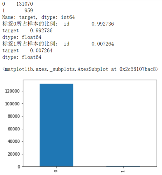
Obviously, this is an extremely unbalanced data classification. For this kind of data, processing methods can refer to The first
The second And so on.

1.1.2 single feature analysis

1. Delete Id and Id number analysis

(1) Merge data
Please note: the purpose of merging data is to view data distribution and do feature engineering. When processing data, training set and test set need to be processed separately.

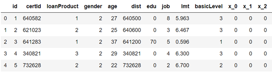
all_data=pd.concat([train_df,test_df])
all_data.head()

(2) View basic data information

all_data.info()

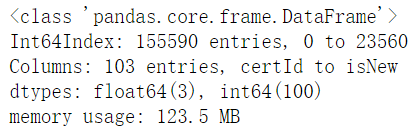
It can be seen from the results that there are 155590 samples in total and 103 columns in total, excluding the id unique value attribute. There are 102 features in total, including 3 in float 64 and 100 in int 64 (including id)

(3) Delete id and certId for visualization and split them

all_data.drop('id',axis=1,inplace=True)
sns.distplot(all_data['certId'])

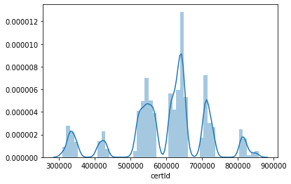
According to the collected data, it can be considered as the first six digits of the ID card, which represents the address code, the administrative division code of the county where the permanent residence is located, the first two digits represent the province, and the third four digits represent the city (1-20, 51-70 refers to provinces and municipalities directly under the central government; 21-50 refers to regions or autonomous prefectures); five or six refers to counties (1-18 refers to municipalities or regions directly under the central government; 21-80 refers to counties; 81-99 refers to counties directly under the central government)
Therefore, the ID number is divided into three parts, and the ID number is deleted

all_data['certId_province']=all_data['certId'].apply(lambda x:str(x)[0:2])
all_data['certId_city']=all_data['certId'].apply(lambda x:str(x)[2:4])
all_data['certId_county']=all_data['certId'].apply(lambda x:str(x)[4:6])

all_data.drop('certId',axis=1,inplace=True)

2. Discrete variable: loan type analysis

all_data['loanProduct'].value_counts().plot.bar()
plt.xlabel('Type of loanProduct')
plt.ylabel('Count')

3. Continuous variables: age analysis

sns.distplot(all_data['age'])

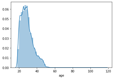
It can be seen from the figure that age attribute does not obey the normal distribution, and there is a serious long tail phenomenon, which needs to be dealt with

3, All codes

import pandas as pd
import numpy as np
import matplotlib.pyplot as plt
import warnings  
import seaborn as sns
warnings.filterwarnings('ignore')  #Ignore warnings
%matplotlib inline
pd.set_option('display.max_columns',None)  #Show all features
import time,datetime

test_df=pd.read_csv(r'C:\Users\Chen\Data mining competition\"Digital financial Cup" of Xiamen International Bank\data\test.csv')
train_df=pd.read_csv(r'C:\Users\Chen\Data mining competition\"Digital financial Cup" of Xiamen International Bank\data\train.csv')
target_df=pd.read_csv(r"C:\Users\Chen\Data mining competition\"Digital financial Cup" of Xiamen International Bank\data\train_target.csv")
y=target_df['target']
submit_id=test_df['id']

all_data=pd.concat([train_df,test_df])
all_data.head()

all_data.drop('id',axis=1,inplace=True)

all_data['certId_province']=all_data['certId'].apply(lambda x:str(x)[0:2])
all_data['certId_city']=all_data['certId'].apply(lambda x:str(x)[2:4])
all_data['certId_county']=all_data['certId'].apply(lambda x:str(x)[4:6])

all_data.drop('certId',axis=1,inplace=True)

bins=[17,30,40,50,120]
labels=['youth','middle age','Prime of life','old age']
all_data['age_cut']=pd.cut(all_data['age'],bins=bins,labels=labels)
all_data.drop('age',axis=1,inplace=True)

all_data['dist_province']=all_data['dist'].apply(lambda x:str(x)[0:2])
all_data['dist_city']=all_data['dist'].apply(lambda x:str(x)[2:4])
all_data['dist_county']=all_data['dist'].apply(lambda x:str(x)[4:6])
all_data.drop('dist',axis=1,inplace=True)

all_data.loc[all_data['edu']==-999,'edu']=80
all_data.loc[all_data['edu']==47,'edu']=50

bins=[0,8,20,100]
labels=['low','in','high']
all_data['lmt_cut']=pd.cut(all_data['lmt'],bins=bins,labels=labels)
all_data.drop('lmt',axis=1,inplace=True)

all_data['certValidStop']=all_data['certValidStop'].apply(lambda x:str(x)[0:10])
all_data['certValidStop']=all_data['certValidStop'].astype(float)
all_data['certValidBegin']=all_data['certValidBegin'].astype(float)
all_data['stop_time']=all_data['certValidStop'].apply(lambda x:time.strftime("%Y--%m--%d %H:%M:%S", time.localtime(x)))
all_data['begin_time']=all_data['certValidBegin'].apply(lambda x:time.strftime("%Y--%m--%d %H:%M:%S",time.localtime(x)))
all_data.drop(['certValidBegin','certValidStop'],axis=1,inplace=True)

all_data['stop_year']=all_data['stop_time'].apply(lambda x:int(x.split(' ')[0].split('--')[0])-70)
all_data['stop_month']=all_data['stop_time'].apply(lambda x:x.split(' ')[0].split('--')[1])
all_data['stop_day']=all_data['stop_time'].apply(lambda x:x.split(' ')[0].split('--')[2])

all_data['begin_year']=all_data['begin_time'].apply(lambda x:int(x.split(' ')[0].split('--')[0])-70)
all_data['begin_month']=all_data['begin_time'].apply(lambda x:x.split(' ')[0].split('--')[1])
all_data['begin_day']=all_data['begin_time'].apply(lambda x:x.split(' ')[0].split('--')[2])
all_data.drop(['stop_time','begin_time'],axis=1,inplace=True)

all_data['residentAddr']=all_data['residentAddr'].apply(lambda x:str(x)[0:6])
all_data['residentAddr']=all_data['residentAddr'].astype(float)
mea=all_data.loc[all_data['residentAddr']!=-999,'residentAddr'].mean()
all_data.loc[all_data['residentAddr']==-999,'residentAddr']=int(mea)
all_data.loc[all_data['highestEdu']==-999,'highestEdu']=0
all_data.loc[all_data['linkRela']==-999,'linkRela']=3

all_data['resident_province']=all_data['residentAddr'].apply(lambda x:str(x)[0:2])
all_data['resident_city']=all_data['residentAddr'].apply(lambda x:str(x)[2:4])
all_data['resident_county']=all_data['residentAddr'].apply(lambda x:str(x)[4:6])
all_data.drop('residentAddr',axis=1,inplace=True)

for i in all_data['ethnic']:
    if i !=0:
        all_data.loc[all_data['ethnic']==i,'ethnic']=1
     
cat_cols=['loanProduct','gender','edu','job','basicLevel','ethnic','highestEdu','linkRela',
          'setupHour','weekday','isNew','certId_province','certId_city','certId_county','age_cut',
          'dist_province','dist_city','dist_county','lmt_cut','stop_year','stop_month','stop_day',
          'begin_year','begin_month','begin_day','resident_province','resident_city','resident_county']
cat_df=all_data[cat_cols]
ori_df=all_data.drop(cat_cols,axis=1)

for i in cat_df.columns:
    cat_df[i]=cat_df[i].astype(str)
cat_dummy=pd.get_dummies(cat_df)
all_feat=pd.concat([cat_dummy,ori_df],axis=1)
all_feat.shape

train=all_feat.iloc[:train_df.shape[0],:]
test=all_feat.iloc[train_df.shape[0]:,:]

from sklearn.model_selection import train_test_split
x_train,x_test,y_train,y_test=train_test_split(train,y)

from xgboost import XGBClassifier
from sklearn.metrics import roc_auc_score,accuracy_score

xgb=XGBClassifier()
xgb.fit(x_train,y_train)

pred=xgb.predict(x_test)
print(accuracy_score(y_test,pred))
roc_auc_score(y_test,pred)

from sklearn.feature_selection import SelectFromModel


select=SelectFromModel(xgb,prefit=True)
new_all_feat=select.transform(all_feat)
new_all_feat.shape

train2=new_all_feat[:train_df.shape[0],:]
test2=new_all_feat[train_df.shape[0]:,:]

x_train2,x_test2,y_train2,y_test2=train_test_split(train2,y)

xgb2=XGBClassifier()
xgb2.fit(x_train2,y_train2)

predict2=xgb2.predict_proba(test2)[:,1]
predict2

submit=pd.DataFrame()
submit['id']=submit_id
submit['target']=predict2
submit=submit.set_index('id')
submit.head()

submit.to_csv(r'C:\Users\Chen\Data mining competition\"Digital financial Cup" of Xiamen International Bank\submit\submit84.csv')

Posted by ahmad03 on Sun, 07 Jun 2020 00:32:29 -0700

Programmer Group