Image classification, according to the different characteristics reflected in the image information, is an image processing method that distinguishes different types of objects. It uses computers to analyze images quantitatively, and classifies each pixel or region in an image into one of several categories to replace human visual interpretation.

12.1 classifier

Classification means that several categories are prepared in advance, and then a target object is assigned to a category according to certain characteristics. Classification can be considered in the following cases:
(1) Image segmentation
(2) Target recognition
(3) Quality inspection
(4) Defect detection
(5) Optical character recognition (OCR)

12.1.1 basic knowledge of classification

1. The significance of classifier
   The classifier is used to assign the target object to one of several categories.
   Feature parameters are stored in feature vector, also known as feature library space.
   A classifier that uses lines or planes for classification is called a linear classifier.
2. Types of classifiers
   (1) MLP classifier based on neural network, especially multilayer perceptual layer
   (2) SVM classifier based on support vector machine
   (3) GMM classifier based on Gaussian mixture model
   (4) k-NN classifier based on k-nearest neighbor
   In addition, halcon also provides a box classifier for binary image classification.
3. General process of image classification
   (1) Prepare a set of sample objects that are known to belong to the same category, extract a set of features from each sample object, and store them in feature vectors
   (2) Create classifier
   condition
   (3) A classifier is trained by the feature vector of the sample. In the training process, a classifier is used to calculate the boundary belonging to a certain category
   (4) Detect the target object and get the feature vector of the object to be detected.
   (5) According to the boundary conditions of the trained classification, the classifier determines which classification the feature of the detected object belongs to.
   (6) Clear classifier
   In general, for a specific classification task, it is necessary to select a suitable set of features, a suitable classifier and a suitable training sample

12.1.2 MLP classifier

MLP is a dynamic classifier based on neural network. MLP classifier can be used in general feature classification, image segmentation, OCR and so on.

MLP (multi-layer perceptron) is also called Artificial Neural Network (ANN). In addition to the input and output layer, there can be multiple hidden layers in the middle. The simplest MLP only contains one hidden layer, which is a three-layer structure, as shown in the following figure: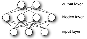

12.1.3 SVN classifier

SVM is support vector machine, which is used to realize data classification. SVM is used for two categories, that is, there are only two categories.

SVM, the full name of which is Support Vector Machine in English and Support Vector Machine in Chinese, was proposed by mathematician Vapnik and others as early as 1963. Prior to the rise of deep learning, SVM was the most classic and popular classification method in machine learning in recent decades.

As shown in the figure below, there are two types of sample data (orange and blue dots), the red line in the middle is the classification hyperplane, and the points on the two dashed lines (three orange dots and two blue dots) are the closest points to the hyperplane, which are the support vectors. In short, as a support vector, sample points are very important, so that other sample points can be ignored. The classification hyperplane is SVM classifier, through which the sample data can be divided into two parts.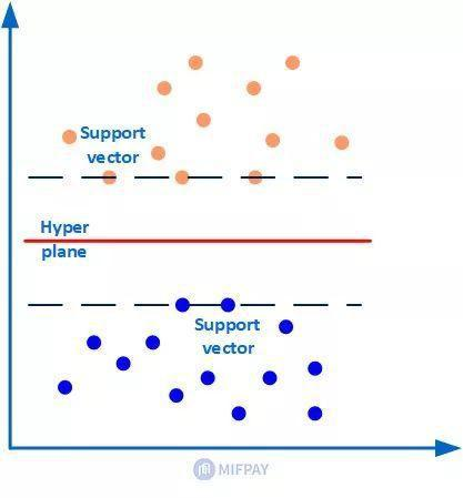

GMM classifier

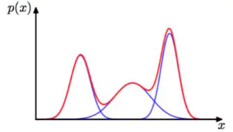
GMM classifier, namely Gaussian mixture model classifier. Gaussian model is a kind of expression that uses Gaussian probability distribution curve, namely normal distribution curve to quantify probability. It can use more than one probability distribution curve.

GMM(Gaussian Mixture Model) refers to the linear superposition and mixing of multiple Gaussian models of the algorithm. Each Gaussian model is called a component. GMM algorithm describes the distribution of data itself.
GMM algorithm is often used in clustering applications, the number of component s can be considered as the number of categories.
Assuming that GMM is a linear superposition of k Gaussian distributions, the probability density function is as follows:

12.1.5 k-NN classifier

k-NN classifier is a simple but powerful classifier, which can store all the training data and classification, and can also classify the new samples based on their adjacent training data.

K-nearest neighbors (knn) is an instance based nonparametric learning algorithm. Here, the input consists of K recent training instances in the dataset, and the output is a class member. The classification principle of a new object is that it is divided into the most of the nearest K neighbors. In particular, when k = 1, the object is assigned to the class of the nearest neighbor. In general, neighbor weight can be assigned to represent the contribution of neighbor to classification. For example, you can take the reciprocal of the distance from an object to each neighbor as its weight. The disadvantage of knn algorithm is that it is sensitive to the local structure of data and easy to over fit data.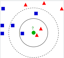

12.1.6 select the appropriate classifier

In most cases, the above four classifiers can be considered. They are flexible and efficient enough. In practice, we can choose the appropriate classifier according to the needs of the project or the limitations of hardware conditions.
(1) MLP classifier: it is fast in classification, but slow in training, low in memory requirements, and supports multi-dimensional feature space. It is especially suitable for scenes requiring fast classification and offline training, but does not support defect detection.
(2) SVM classifier: the speed of classification and detection is fast. When the vector dimension is low, it is the fastest, but slower than MLP classifier, although its training speed is much faster than MLP classifier. Its memory usage depends on the number of samples. If there are a large number of samples, such as character library, which need training, the classifier will become very large.
(3) GMM classifier: the training speed and detection speed are very fast, especially when there are few categories. It supports anomaly detection, but it is not suitable for high-dimensional feature detection.
(4) kNN classifier: the training speed is very fast, and the classification speed is slower than MLP classifier. It is suitable for defect detection and multi-dimensional feature classification, but it needs more memory.

In addition to the classifier, the selection of features and training samples will also affect the classification results. When the classification results are not ideal, these two factors can be adjusted. If the training sample already contains all the relevant features of the target object, but the classification result is still not ideal, then another classifier can be considered.

12.1.7 selection of appropriate features

What kind of feature to choose depends on what the detected object is and what the classification requirements are.

12.1.8 select appropriate training samples

~

12.2 classification of features

The steps of classification are: first, to create a suitable classifier; then, to investigate the characteristics of the object, to add the appropriate feature vector to the texture classifier; finally, to use the sample data for training, so that the classifier can learn some classification rules. In the detection, the target corresponding to the feature value of the classifier is extracted, and the trained classifier is used for classification. After using the classifier, clear it from memory.

12.2.1 general steps

(1) Identify the categories, and collect the appropriate image as the sample data set according to the categories.
(2) Create classifier
(3) Get the eigenvectors of the samples with clear categories
(4) Add these samples to the classifier by category number
(5) Training classifier
(6) Save classifier (for subsequent calls)
(7) Obtain the eigenvectors of the tested object of unknown classification, which should be the eigenvectors used in the previous training of classifier
(8) Classify the feature vector of the tested object
(9) Clear classifier from memory

12.2.2 MLP classifier

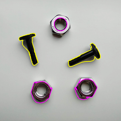
*Close the current window
dev_close_window ()
*Create a new window
dev_open_window (0, 0, 512, 512, 'black', WindowHandle)
*Set how shapes are drawn
dev_set_draw ('margin')
dev_set_line_width (3)
*establish mlp Classifier, number of features is1，The output class is2Output method selection'softmax'For classification
create_class_mlp (1, 1, 2, 'softmax', 'normalization', 3, 42, MLPHandle)
*Creating the corresponding relationship between training sample image and its classification
*One to one correspondence between image and classification name
FileNames := ['m1','m2','m3','m4']
Classes := [0,0,1,1]
for J := 0 to |FileNames| - 1 by 1
	*Read training image
	read_image (Image, 'data/' + FileNames[J])
	dev_display (Image)
	*Image segmentation
    rgb1_to_gray (Image, GrayImage)
    threshold (GrayImage, darkRegion, 0, 105)
    connection (darkRegion, ConnectedRegions)
    select_shape (ConnectedRegions, SelectedRegions, 'area', 'and', 2000, 99999)
	fill_up (SelectedRegions, Objects)
	dev_display (Objects)
	disp_message (WindowHandle, 'Add Sample ' + J + ', Class Index ' + Classes[J], 'window', 10, 10, 'black', 'true')
	*Objects to be split objects Add the classification corresponding to the classifier Classes[J]in
	count_obj (Objects, Number)
    *Extract feature (roundness)
    for N := 1 to Number by 1
      select_obj (Objects, Region, N)
      circularity (Region, Circularity)
      add_sample_class_mlp (MLPHandle, Circularity,Classes[J])
    endfor
    stop()
	disp_continue_message (WindowHandle, 'black', 'true')
endfor
dev_clear_window ()
disp_message (WindowHandle, 'Training...', 'window', 10, 10, 'black', 'true')
*train mlp classifier 
train_class_mlp (MLPHandle, 200, 1, 0.01, Error, ErrorLog)
clear_samples_class_mlp (MLPHandle)

*Read the input image to be detected
read_image (testImage, 'data/m5')
rgb1_to_gray (testImage, GrayTestImage)
*Image segmentation
threshold (GrayTestImage, darkTestRegion, 0, 105)
connection (darkTestRegion, ConnectedTestRegions)
select_shape (ConnectedTestRegions, SelectedTestRegions, 'area', 'and', 1500, 99999)
fill_up (SelectedTestRegions, testObjects)
*Objects to be split objects Classify
count_obj (testObjects, Number)
Classes := []
Colors := ['yellow','magenta']
dev_set_colored (6)
dev_display (testImage)
*Extract feature (roundness)
for J := 1 to Number by 1
    select_obj (testObjects, singleRegion, J)
    circularity (singleRegion, Circularity)
    classify_class_mlp (MLPHandle, Circularity, 1, Class, Confidence)
    Classes := [Classes,Class]
    dev_set_color (Colors[Classes[J-1]])
    dev_display (singleRegion)
endfor

*eliminate MLP Classifiers, freeing memory
clear_class_mlp (MLPHandle)

12.2.3 SVM classifier

Pay attention to adjust the corresponding parameters

12.2.4 GMM classifier

Pay attention to adjust the corresponding parameters

12.2.5 k-NN classifier

Pay attention to adjust the corresponding parameters

12.3 optical character recognition

OCR (optical character recognition) is a further classification method for character recognition. The first step of recognition is to extract the independent character region from the image, and then assign it to a character type. MLP, SVM and k-NN classifiers can be used in OCR.

12.3.1 general steps

OCR detection is divided into offline training and online detection.

1. off-line training
   The offline part generally refers to the character training process, including the following steps.
   (1) Read the sample image and segment the known characters in the sample. The unit of segmentation is the surrounding area of a single character
   (2) Store the segmented area and the corresponding character name in the training file
   (3) Check the correspondence in the training file, that is, the names of images and characters should correspond one by one
   (4) Training classifier
   (5) Save classifier
   (6) Clear classifier
2. Online detection
   OCR in the online part refers to the detection of characters, that is, classification. The general process is as follows.
   (1) Read classifier.
   (2) The characters to be detected are segmented to extract independent character regions.
   (3) Classifiers are used to classify character regions.
   (4) Clear the classifier.

12.3.2 OCR example

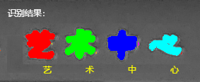
dev_close_window()
read_image (Image, 'data/modelWords')
get_image_size(Image,width,height)
dev_open_window (0, 0, width, height, 'black', WindowHandle)
rgb1_to_gray (Image, GrayImage)  
gen_empty_obj (EmptyObject)
for Index := 1 to 4 by 1
	disp_message (WindowHandle, 'Please select a single Chinese character area and right-click to confirm:','window', 12, 12, 'yellow', 'false')
	draw_rectangle1 (WindowHandle, Row1, Column1, Row2, Column2)
	 **Generate the corresponding rectangle according to the drawn rectangle
	gen_rectangle1 (Rectangle, Row1, Column1, Row2, Column2)
	reduce_domain (GrayImage, Rectangle, ImageReduced1)
	 *Threshold processing
	threshold (ImageReduced1, Region1, 128, 255)
	 *Ready to receive all extracted character regions
	concat_obj (EmptyObject, Region1, EmptyObject)
endfor
words:=['art','art','in','heart']
*sort
sort_region (EmptyObject, SortedRegions1, 'character', 'true', 'row')
for Index1:=1 to 4 by 1
select_obj (SortedRegions1, ObjectSelected1, Index1)
append_ocr_trainf (ObjectSelected1, Image, words[Index1-1], 'data/yszx.trf')
endfor
read_ocr_trainf_names ('data/yszx.trf', CharacterNames, CharacterCount)
create_ocr_class_mlp (50, 60, 'constant', 'default', CharacterNames, 80, 'none', 10, 42, OCRHandle)
trainf_ocr_class_mlp (OCRHandle, 'data/yszx.trf', 200, 1, 0.01, Error, ErrorLog)
write_ocr_class_mlp (OCRHandle, 'data/yszx.omc')
*Import another chart for testing
read_image (ImageTest, 'data/testWords.jpg')
rgb1_to_gray (ImageTest, Image1)
threshold (Image1, testwordregion, 125, 255)
*Segmentation of character regions that meet the requirements
connection (testwordregion, ConnectedwordRegions)
*Filter eligible character shape regions
select_shape (ConnectedwordRegions, SelectedwordRegions, 'area', 'and', 700, 2500)
*Left to right, sort
sort_region (SelectedwordRegions, SortedRegions2, 'upper_left', 'true', 'column')
count_obj(SortedRegions2, Number)
*Start character recognition
read_ocr_class_mlp ('data/yszx.omc', OCRHandle1)
do_ocr_multi_class_mlp (SortedRegions2, Image1, OCRHandle1, Class, Confidence)
*Show results
disp_message(WindowHandle, 'Identification results:', 'image', 10, 10, 'white', 'false')
for i:=1 to 4 by 1
	disp_message(WindowHandle, Class[i-1], 'image', 90, 60*i, 'yellow', 'false')
endfor