1: Random Initialization
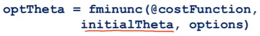
When we use gradient descent or other advanced optimization algorithms, we need to select some initial values for the parameter theta.For advanced optimization algorithms, we assume by default that we have set the initial value for the variable theta:
Similarly, for the gradient descent method, we also need to initialize theta.Then we can minimize the cost function J by descending the gradient step by step, so how do we initialize theta?
(1) Setting theta all to 0--not applicable in neural networks
Although this can be used in logistic regression.But it does not play a role in the actual training of neural networks.
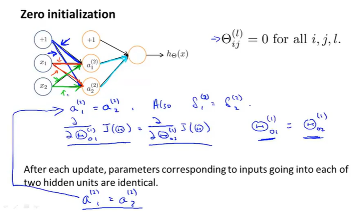
If we initialize all theta zeros (all equal):
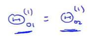
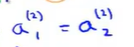
The inputs for each hidden unit are essentially the same:
So the partial derivatives are the same.
When we just set a step, after each parameter update.The weight of each hidden unit is also consistent.
This means that this neural network can't compute a good function. When we have many hidden cells, all the hidden cells are calculating the same characteristics and taking the same function as input.- High redundancy.So no matter how many output units follow, you end up with only one feature, which prevents the neural network from learning something interesting
(2) Random Initialization - Solving the above problem where all weights are equal (symmetric problem)
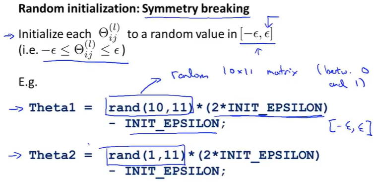
(3) Code implementation
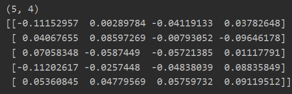
def rand_initiation(l_in,l_out):    #For adjacent layers
    w = np.zeros((l_out,l_in+1))  #Need to add the paranoid unit weight of the previous layer
    eps_init = 0.12 #Near 0, keep at-εreachεBetween
    w = np.random.rand(l_out,l_in+1)*2*eps_init-eps_init
    return w
w = rand_initiation(3,5)
print(w.shape)
print(w)
Or use the following method for random initialization:
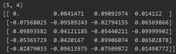
def debug_initialize_weights(fan_in,fan_out):
    w = np.zeros((fan_out,1+fan_in))
    w = np.sin(np.arange(w.size)).reshape(w.shape) / 10  #Using sin guarantees that values are between (-1, 1) and divided by 10, the values are initialized between (-0.1, 0.1)
    return w
w = debug_initialize_weights(3,5)
print(w.shape)
print(w)
2: Gradient Test--Ensure the correctness of the reverse propagation code we implemented
(1) Problems Existing in Reverse Propagation
Previously, we learned how to use the forward and reverse propagation algorithms in the neural network to calculate derivatives, but the back propagation algorithm has many details, is complex to implement, and has a bad feature:
When reverse propagation works with gradient descent or other algorithms, there may be some undetectable errors, meaning that although the cost function J appears to be decreasing, the final result may not be the optimal solution.The error will be one magnitude higher than if there were no bugs.And we probably don't know that the problem we're having is caused by Bug.
Solution: - Gradient test
Almost all of these problems can be solved.Gradient tests are performed almost at the same time as all reverse propagation or other similar gradient descent algorithms are used.He will ensure that forward propagation is completely correct and that backward propagation is already complete.
Can be used to verify that the code you write actually correctly calculates the derivative of the cost function J
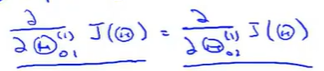
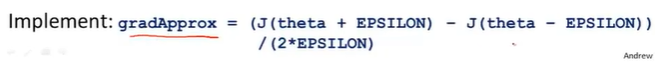
(2) Definition method for solving derivatives
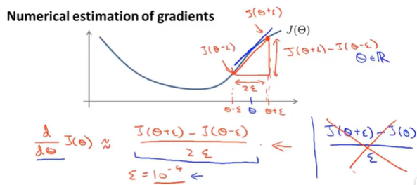
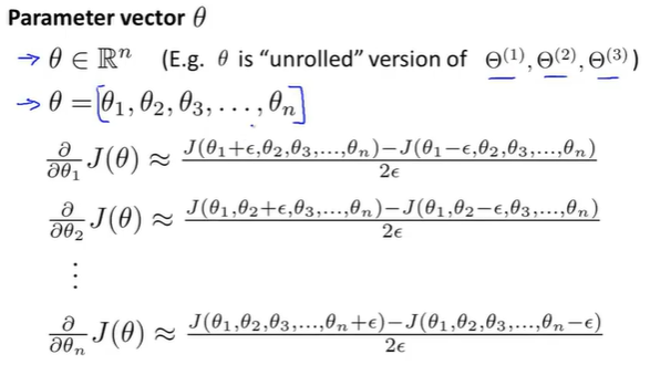
When theta is a vector, we need to check the partial derivatives:
(3) algorithm implementation
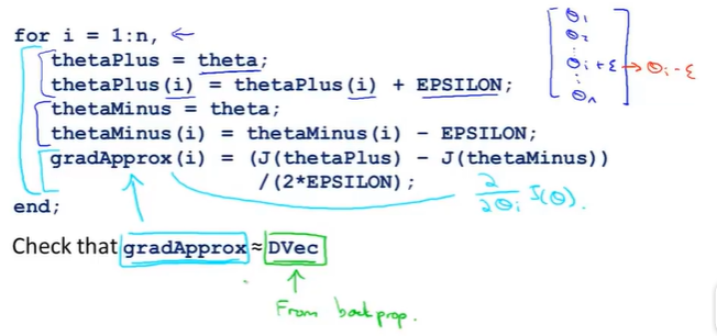
n represents the theta parameter dimension, and we perform the derivation above for each theta_i.We then test whether the derivatives we use to define them are close (several decimal differences) or equal to those we use reverse propagation.Then we can be sure that the implementation of reverse propagation is correct.J( theta) can be optimized very well
Note: We only need to use a gradient test to verify that the derivatives obtained by our back-propagation algorithm are correct.If it is correct, then we need to turn off gradient testing for later learning (because gradient testing is computationally intensive and slow)
(4) Code implementation
def compute_numerial_gradient(cost_func,theta): #Used to calculate gradients
    numgrad = np.zeros(theta.size)  #Preserve Gradient
    perturb = np.zeros(theta.size)  #Keeping every calculated gradient, theta_j of only one dimension subtracts epsilon
    e = 1e-4

    for i in range(theta.size):
        perturb[i] = e
        J_1 = cost_func(theta-perturb)
        J_2 = cost_func(theta+perturb)

        numgrad[i] = (J_2-J_1)/(2*e)
        perturb[i] = 0  #Modified location data needs to be restored

    return numgrad
def check_gradients(lamda):
    #Because a real training set has too much data, here we randomly generate some small-scale data for statistical testing.
    input_layer_size = 3    #input layer
    hidden_layer_size = 5   #Hidden Layer
    num_labels = 3          #output layer---Number of Classifications

    m = 5   #Number of data sets

    #Initialization Weight Parameter
    theta1 = debug_initialize_weights(input_layer_size,hidden_layer_size)
    theta2 = debug_initialize_weights(hidden_layer_size,num_labels)

    #Similarly: Initialize some training set X and tag value y
    X = debug_initialize_weights(input_layer_size - 1,m)    #The training set is m rows, input_layer_size column
    y = 1 + np.mod(np.arange(1,m+1),num_labels) #Remaining Category 1->num_labels
    encoder = OneHotEncoder(sparse=False)   #sparse=True Represents the format of the encoding, defaulting to True,Is the sparse format, specified False Then you don't need to toarray() Yes
    y_onehot = encoder.fit_transform(np.array([y]).T)   #y needs to be a column vector

    #Expand parameters
    theta_param = np.concatenate([np.ravel(theta1),np.ravel(theta2)])

    #1.Using derivative definition to derive
    def cost_func(theta_p):
        return cost(theta_p,input_layer_size,hidden_layer_size,num_labels,X,y_onehot,lamda)  #Cost Function Partial Derivative J( theta)

    numgrad = compute_numerial_gradient(cost_func,theta_param)
    #2.Derivation using reverse propagation
    J,grad = backporp(theta_param,input_layer_size,hidden_layer_size,num_labels,X,y_onehot,lamda)
    print(np.c_[grad,numgrad,grad-numgrad])   #Output of results, comparison
check_gradients(0) #Modifying lamda is still close
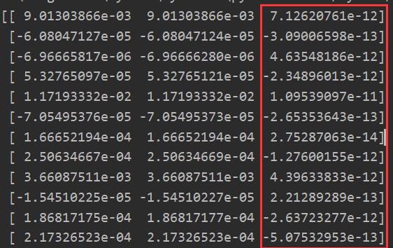
It can be seen that the derivative we get by using the derivative definition is close to the derivative we get by using reverse propagation!!!
So: our back propagation algorithm is correct!!!