python data analysis personal study notes-directory index
Chapter 9 - Random Forest Project Actual Warfare - Temperature Prediction (2/2)
Chapter 8 has explained the basic principles of random forests. From a practical point of view, this chapter will complete the task of temperature prediction with Python toolkit, which involves several modules, including random forest modeling, feature selection, efficiency comparison, parameter tuning, and so on.This is a really long example, divided into three sections.This is the second article.
9.2 Impact of Data and Features on Results
With the questions posed in the previous section, re-reading the larger data, or maintaining the same task, requires observing the impact of the selection of data volume and characteristics on the results, respectively.
1 # Import Toolkit
2 import pandas as pd 3 4 # Read data 5 features = pd.read_csv('data/temps_extended.csv') 6 features.head(5) 7 8 print('Data Size',features.shape)
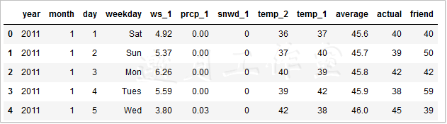
Data Size (2191, 12)
In the new data, the size of the data has changed, expanding to 2191, and incorporating the following three new weather features.
- ws_1: Wind speed for the previous day.
- prcp_1: Precipitation from the previous day.
- snwd_1: The snow depth of the previous day.
With new features, you can visualize your drawings.
 1 # Set the overall layout
 2 fig, ((ax1, ax2), (ax3, ax4)) = plt.subplots(nrows=2, ncols=2, figsize = (15,10))  3 fig.autofmt_xdate(rotation = 45)  4  5 # Average Maximum Temperature  6 ax1.plot(dates, features['average'])  7 ax1.set_xlabel(''); ax1.set_ylabel('Temperature (F)'); ax1.set_title('Historical Avg Max Temp')  8  9 # wind speed 10 ax2.plot(dates, features['ws_1'], 'r-') 11 ax2.set_xlabel(''); ax2.set_ylabel('Wind Speed (mph)'); ax2.set_title('Prior Wind Speed') 12 13 # precipitation 14 ax3.plot(dates, features['prcp_1'], 'r-') 15 ax3.set_xlabel('Date'); ax3.set_ylabel('Precipitation (in)'); ax3.set_title('Prior Precipitation') 16 17 # Accumulated snow 18 ax4.plot(dates, features['snwd_1'], 'ro') 19 ax4.set_xlabel('Date'); ax4.set_ylabel('Snow Depth (in)'); ax4.set_title('Prior Snow Depth') 20 21 plt.tight_layout(pad=2)
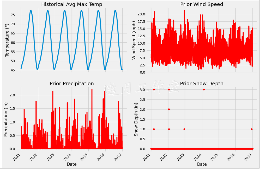
3 new features are added to make the visualization easy to understand. On the one hand, the purpose of visualization is to observe the features, on the other hand, to consider whether there is a problem with their values, because the data you usually get is not so clean. Of course, the data in this example is still very friendly and can be used directly.
9.2.1 Feature Engineering
In the process of data analysis and feature extraction, the starting point is to select as many valuable features as possible, because the more information that can be obtained in the initial stage, the more information that can be used in modeling.As you go deeper into the machine learning project, you will find a phenomenon: after modeling, you will think of some data features that can be used, then go back to preprocess and extract the data signs, and then re-conduct the modeling analysis.
After repeatedly extracting features, the most common thing to do is to make experimental comparisons, but if the amount of data is very large, it will take relatively more time to extract features at one time. Therefore, it is recommended that you improve the pre-processing and feature extraction as much as possible at the beginning, and you can also make several more schemes for comparison and analysis.
For example, in this data, there are complete date features, it is clear that weather changes are related to seasonal factors, but in the original dataset, there are no indicators of seasonal characteristics, so you can create a seasonal variable yourself as a new feature, which will help both modeling and analysis.
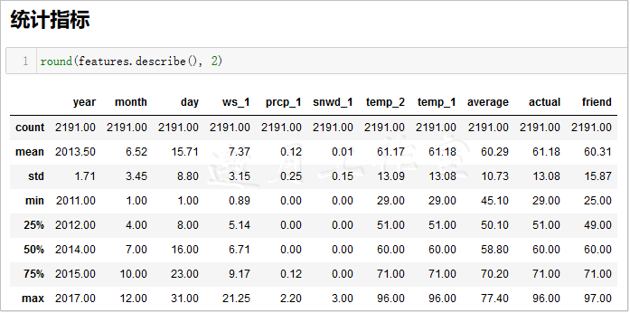
 1 # Create a seasonal variable
 2 seasons = []  3  4 for month in features['month']:  5 if month in [1, 2, 12]:  6 seasons.append('winter')  7 elif month in [3, 4, 5]:  8 seasons.append('spring')  9 elif month in [6, 7, 8]: 10 seasons.append('summer') 11 elif month in [9, 10, 11]: 12 seasons.append('fall') 13 14 # With the seasons we can analyze more 15 reduced_features = features[['temp_1', 'prcp_1', 'average', 'actual']] 16 # reduced_features=reduced_features.copy() 17 reduced_features['season'] = seasons 18 19 ####reduced_features['season']=None #Add a new column 20 21 # reduced_features=reduced_features.copy() 22 23 # for k in range(0,len(seasons)): 24 # reduced_features.loc[k,'season']=seasons[k] 25 26 # reduced_features.loc[:, 'season'] = '30' #Set an Integer Column Value 27 ####print(reduced_features.columns) #Column Name All 28 # print(reduced_features.columns[4]) #Column Name season 29 ####print(reduced_features.iloc[:,4]) #Column 5 Values 30 # print(reduced_features.iloc[:,3]) #Column 4 Values 31 32 33 # for label, content in reduced_features.items(): 34 # print('label:', label) 35 # print('content:', content, sep='\n') 36 37 38 print(round(reduced_features.describe(),2)) 39 # print(len(reduced_features)) ##2191 40 # print(reduced_features.shape[1]) #Column Number 5 41 # print(reduced_features.shape[0]) #Number of rows 2191 42 # print(reduced_features.columns[4]) #Column Name season 43 # print(reduced_features.loc[0,'season']) #Can't find column?? KeyError: 'season' 44 print(reduced_features.loc[:,'season']) #Can't find column?? KeyError: 'season' 45 # https://pandas.pydata.org/pandas-docs/stable/reference/api/pandas.DataFrame.loc.html 46 # print(reduced_features.loc['season'])
Note here: Line 17 raises a warning:
/* d:\tools\python37\lib\site-packages\ipykernel_launcher.py:16: SettingWithCopyWarning:
A value is trying to be set on a copy of a slice from a DataFrame.
Try using .loc[row_indexer,col_indexer] = value instead
See the caveats in the documentation: https://pandas.pydata.org/pandas-docs/stable/user_guide/indexing.html#returning-a-view-versus-a-copy
app.launch_new_instance()
*/
Two solutions:
 1 #Two scenarios:
 2 #1,plus copy  3  4 reduced_features=reduced_features.copy()  5 reduced_features['season'] = seasons  6  7 #2,Use loc assignment  8  9 # reduced_features.loc[:,'season'] = seasons 10 11 #After slicing list Data storage df in 12 for k in range(0,len(seasons)): 13 reduced_features.loc[k,'season']=seasons[k]
With seasonal characteristics, what if you want to see how these characteristics change in different seasons?Here we recommend a very practical drawing function, pairplot(), which requires the installation of the Seaborn toolkit (pip install seaborn), which is equivalent to encapsulating on the basis of Matplotlib, making it easier to use:
 1 Import seaborn Toolkit
 2 import Seaborn as SNS 3 sns.set (style="ticks", color_codes=True); 45 #Choose your favorite color template 6 palette = sns.xkcd_palette (['dark blue','dark green','gold','orangeange']) 7 8 #Paiplotplotplotplot 9 ## help (sns.pairplot) 10 # https://seaborn.pydata.org/generated/seaborn.pydata.org/generated/seaborn.plotplotplotplot pair.html#seaborn.pairplotplotplotplotplot11 #default parameter 12 # sns.pair (reduced_features, hue=None, hue_order=None, Nonplotplot=None, palette=None, vars=e, vars=vars=None, x_vars=None, y_vars=None, y_vars=None, 13 \### scatter # scatter scatter'scatter', diag_kind='auto', markers=None, height=2.5, aspect=1,14# corner=False, dropna=True, dropna=True, plot_kws=None, diag_kws=None, plot_kws=None, diag_kws=None, grid_kws=None, size=None) 15 16 sns.pairplot (reduced_features, hue ='season', diag_type='reg', palette= palette, plot_kws=dict (alpha = 0.7), 17 diag_kws=kws=dict (shade=True); 18 19.reduced plot (reduced features, dropplot_features, dropna=True, dropna=True, dropdropdropdropdropna = True, huhuhuhuhuhue =True, True=True, g_type='kde', palette= palette,Plot_kws=dict (alpha=0.7), 20 diag_kws=dict (shade=True));
The source code keeps making mistakes, read the official documents, and there is no solution.
https://seaborn.pydata.org/generated/seaborn.pairplot.html#seaborn.pairplot
d:\tools\python37\lib\site-packages\statsmodels\nonparametric\bandwidths.py in select_bandwidth(x, bw, kernel)
    172         # eventually this can fall back on another selection criterion.
    173         err = "Selected KDE bandwidth is 0. Cannot estimate density." --> 174 raise RuntimeError(err) 175 else: 176 return bandwidth RuntimeError: Selected KDE bandwidth is 0. Cannot estimate density.
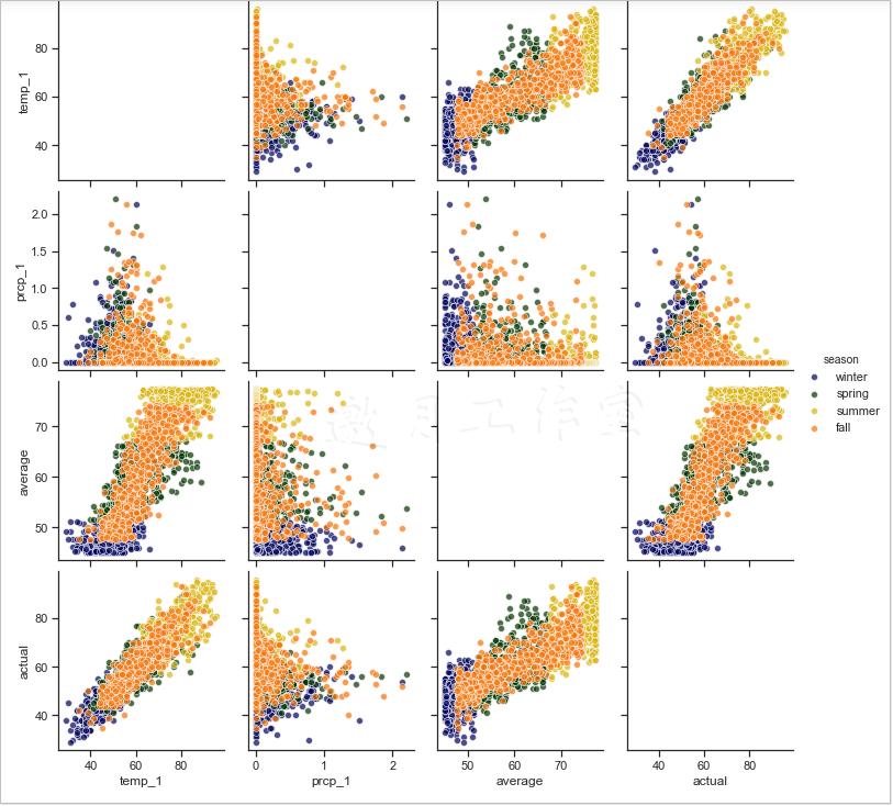
Note: Diagonal graphs are not generated.
The above output shows that the x-axis and y-axis are temp_1, prcp_1, average and actual. Points with different colors represent different seasons (set by the hue parameter). The x-axis and y-axis on the main diagonal are all numeric distributions with the same characteristics in different seasons. Other locations use scatterplots to show the relationship between the two features, for example, lower left.Angle temp_1 and actual show strong correlation.
9.2.2 Data Volume Impact Analysis on Results
The next step is a series of comparative experiments. The first question is whether the results will change when the data increases using the same method of modeling.Or slice the new dataset first:
 1 #Unique Hot Coding
 2 features = pd.get_dummies(features) 34 #Extract features and labels 5 labels = features['actual'] 6 features = features.drop('actual',Axis = 1) 78 #Feature name with alternate 9 feature_list = list (features.columns) 1011 #Convert to required format 12 import numpy as NP 13 14 features = np.array (features) 15 labels = np.array (labels) 1617 #Dataset sliced 18 from sklearn.model_import train_test_19 20_features, test_features, train_labels,Test_labels = train_test_split (features, labels, 21 test_size = 0.25, random_state = 0) 2223 prints ('training set features:', train_features.shape') 24 prints ('training set labels:', train_labels.shape') 25 prints ('test set features:', test_features.shape') 26 prints ('test set labels:', test_labels.shape)
Training set characteristics: (1643, 17) Training set label: (1643,) Test set characteristics: (548, 17) Test Set Label: (548,)
The new dataset consists of 1643 training samples and 548 test samples.For comparison experiments, the same test set is used to compare the results, and since a new Notebook snippet is reopened, the same preprocessing is performed again on older datasets with fewer samples:
 1 #Toolkit Import
 2 import pandas as PD 3 4 #In order to eliminate the effect of the number of features on the results, the only feature uniform here is feature 5 original_feature_indices = [feature_list.index(feature) for feature in 6 feature_list if feature not in 7 ['ws_1','prcp_1','snwd_1']] 8 9 #Read the old dataset 10 original_features = pd.read_csv('data/temps.csv') 11 12 original_features = pd.get_dummies(original_features) 13 14 import numpy as np 15 16 #Data and label conversion 17 original_labels = np.array (original_features['actual']) 18 19 original_features= original_features.drop ('actual', features)Axis = 1) 2021 original_feature_list = list (original_features.columns) 2223 original_features = np.array (original_features) 2425 #dataset slicing 26 from sklearn.model_selection import_train_test_split 27 28 original_train_features, original_test_features, original_train_labels, original_test_labels = train_test_split (original_features,Original_labels, test_size = 0.25, random_state = 42) 2930 #The same tree model is modeled 31 from sklearn.ensemble import RandomForestRegressor 3233 #The same parameters as random seed 34 RF = RandomForestRegressor (n_estimators= 100, random_state = 0) 3536 #The training set here uses 37 rf.fit (original_train_features, features) of the old dataset.Original_train_labels); 3839 #For fairness in testing results and consistency of test sets, select test set 40 predictions = rf.predict (test_features[:, original_feature_indices]) 4142 #Calculate average temperature error 43 errors = ABS (predictions - test_labels) 4445 ('average temperature error:',Round (np.mean (errors), 2),'degrees.') 46 47 # MAPE 48 MAPE = 100 * (errors / test_labels) 49 50 #Accuracy here for easy observation, we subtract the error with 100, and hope that the higher the value, the better 51 accuracy = 100 - np.mean (mape) 52 ('Accuracy:', round (accuracy, 2),'%.')
Average temperature error: 4.67 degrees.
Accuracy: 92.2 %.
The above output shows an average temperature error of 4.67, which is the result when the number of samples is small. Let's see if the effect increases with the number of samples:
 1 from sklearn.ensemble import RandomForestRegressor
 2  3 # Remove new features to ensure consistent data characteristics  4 original_train_features = train_features[:,original_feature_indices]  5  6 original_test_features = test_features[:, original_feature_indices]  7  8 rf = RandomForestRegressor(n_estimators= 100 ,random_state=0)  9 10 rf.fit(original_train_features, train_labels); 11 12 # Forecast 13 baseline_predictions = rf.predict(original_test_features) 14 15 # Result 16 baseline_errors = abs(baseline_predictions - test_labels) 17 18 print('Average temperature error:', round(np.mean(baseline_errors), 2), 'degrees.') 19 20 # (MAPE) 21 baseline_mape = 100 * np.mean((baseline_errors / test_labels)) 22 23 # accuracy 24 baseline_accuracy = 100 - baseline_mape 25 print('Accuracy:', round(baseline_accuracy, 2), '%.')
Average temperature error: 4.2 degrees.
Accuracy: 93.12 %.
You can see that when the amount of data increases, the average temperature error is 4.2, the effect has some improvement, which is also in line with the actual situation. In machine learning tasks, the larger the amount of data, the better, on the one hand, to enable the machine to learn more fully, on the other hand, to reduce the risk of fitting.
9.2.3 Effect of Number of Features on Results
The following is a comparison of the impact of the number of features on the results. No new weather features were added to the previous two comparisons. This time, precipitation, wind speed, and snow cover were added to the dataset to see how this works:
 1 # Ready to add new features
 2 from sklearn.ensemble import RandomForestRegressor  3  4 rf_exp = RandomForestRegressor(n_estimators= 100, random_state=0)  5 rf_exp.fit(train_features, train_labels)  6  7 # Same Test Set  8 predictions = rf_exp.predict(test_features)  9 10 # Assessment 11 errors = abs(predictions - test_labels) 12 13 print('Average temperature error:', round(np.mean(errors), 2), 'degrees.') 14 15 # (MAPE) 16 mape = np.mean(100 * (errors / test_labels)) 17 18 # See how much you've improved 19 improvement_baseline = 100 * abs(mape - baseline_mape) / baseline_mape 20 print('Increased model performance with more features:', round(improvement_baseline, 2), '%.') 21 22 # accuracy 23 accuracy = 100 - mape 24 print('Accuracy:', round(accuracy, 2), '%.')
Average temperature error: 4.05 degrees.
The effect of the model is improved with more features: 3.34%.
Accuracy: 93.35 %.
The overall effect of the model has been slightly improved, you can see that each improvement in the modeling process will result in a partial improvement of the results, do not underestimate these, cumulative results are great.
While continuing to study the indicator of the importance of features is only for reference, there are also empirical values for reference in the industry:
 1 # Feature name
 2 importances = list(rf_exp.feature_importances_)
 3
 4 # Name, numeric combination
 5 feature_importances = [(feature, round(importance, 2)) for feature, importance in zip(feature_list, importances)]
 6
 7 # sort
 8 feature_importances = sorted(feature_importances, key = lambda x: x[1], reverse = True)
 9
10 # Print out
11 [print('Features: {:20} Importance: {}'.format(*pair)) for pair in feature_importances];
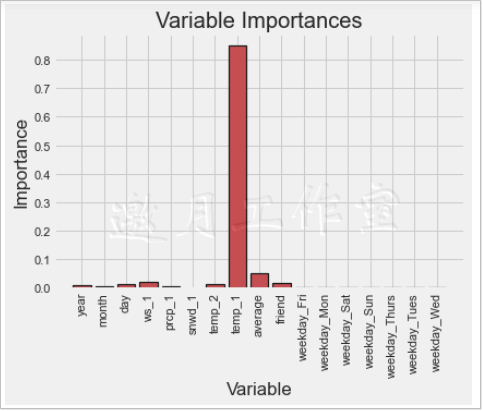
Feature: temp_1 Importance: 0.85
 Feature: average importance: 0.05
 Feature: ws_1 Importance: 0.02
 Feature: friend importance: 0.02
 Feature: year importance: 0.01
 Feature: month importance: 0.01
 Feature: day Importance: 0.01
 Feature: Importance of prcp_1: 0.01
 Feature: temp_2 Importance: 0.01
 Feature: snwd_1 Importance: 0.0
 Feature: weekday_Fri Importance: 0.0
 Feature: weekday_Mon Importance: 0.0
 Feature: weekday_Sat Importance: 0.0
 Feature: weekday_Sun Importance: 0.0
 Feature: weekday_Thurs Importance: 0.0
 Feature: weekday_Tues Importance: 0.0
 Feature: weekday_Wed Importance: 0.0
After sorting the importance of each feature, the results are printed out, followed by temp_1 and average. Wind speed ws_1 is also on the list, but the impact is slightly smaller. A long series of data may seem inconvenient or more clearly shown in a chart.
 1 # Specify Style
 2 plt.style.use('fivethirtyeight')
 3
 4 # Specify location
 5 x_values = list(range(len(importances)))
 6
 7 # Mapping
 8 plt.bar(x_values, importances, orientation = 'vertical', color = 'r', edgecolor = 'k', linewidth = 1.2)
 9
10 # x Axis names have to be written vertically
11 plt.xticks(x_values, feature_list, rotation='vertical')
12
13 # Map Name
14 plt.ylabel('Importance'); plt.xlabel('Variable'); plt.title('Variable Importances');
Although the importance of each feature can be represented by a column chart, it is somewhat blurry to choose how many features to model.The cumsum() function can be used to sort the features by their importance before calculating their cumulative values, such as cumsum([1,2,3,4]) which means the cumulative value (1,3,6,10).Then set a threshold, usually 95 percent, to see how many features are needed to add up before the added value of feature importance exceeds that threshold, and use them as filtered features:
 1 # Sort features
 2 sorted_importances = [importance[1] for importance in feature_importances]
 3 sorted_features = [importance[0] for importance in feature_importances]
 4
 5 # Accumulated importance
 6 cumulative_importances = np.cumsum(sorted_importances)
 7
 8 # Draw a line chart
 9 plt.plot(x_values, cumulative_importances, 'g-')
10
11 # Draw a red dashed line, 0.95 that
12 plt.hlines(y = 0.95, xmin=0, xmax=len(sorted_importances), color = 'r', linestyles = 'dashed')
13
14 # X axis
15 plt.xticks(x_values, sorted_features, rotation = 'vertical')
16
17 # Y Axis and Name
18 plt.xlabel('Variable'); plt.ylabel('Cumulative Importance'); plt.title('Cumulative Importances');
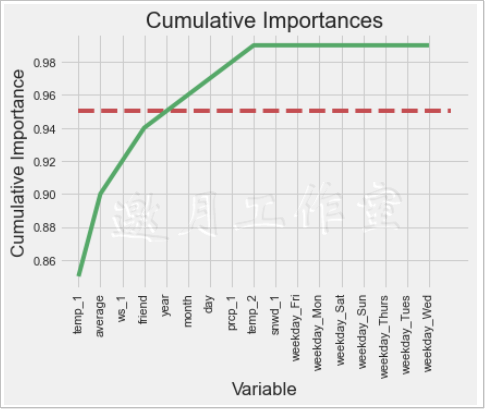
The output shows that when the fifth feature appears, its total cumulative value exceeds 95%, so a comparative experiment can be carried out next. What happens if only the five features are modeled?What about time efficiency?
1 # Look at a few features
2 print('Number of features for 95% importance:', np.where(cumulative_importances > 0.95)[0][0] + 1)
3
4 #Number of features for 95% importance: 5
 1 # Select these features
 2 important_feature_names = [feature[0] for feature in feature_importances[0:5]]
 3 # Find their names
 4 important_indices = [feature_list.index(feature) for feature in important_feature_names]
 5
 6 # Re-create training set
 7 important_train_features = train_features[:, important_indices]
 8 important_test_features = test_features[:, important_indices]
 9
10 # Data Dimension
11 print('Important train features shape:', important_train_features.shape)
12 print('Important test features shape:', important_test_features.shape)
Important train features shape: (1643, 5)
Important test features shape: (548, 5)
 1 # Retraining model
 2 rf_exp.fit(important_train_features, train_labels);
 3
 4 # Same Test Set
 5 predictions = rf_exp.predict(important_test_features)
 6
 7 # Assessment Results
 8 errors = abs(predictions - test_labels)
 9
10 print('Average temperature error:', round(np.mean(errors), 2), 'degrees.')
11
12 mape = 100 * (errors / test_labels)
13
14 # accuracy
15 accuracy = 100 - np.mean(mape)
16 print('Accuracy:', round(accuracy, 2), '%.')
Average temperature error: 4.11 degrees.
Accuracy: 93.28 %.
The miracle does not seem to be happening, thought it might be better, but it has actually decreased a little, either because the tree model itself has passive skills for feature selection or because the remaining 5% of the features do contribute.Although the effect of the model has not been improved, you can also see if there is any improvement in time efficiency:
 1 # Time to calculate
 2 import time
 3
 4 # This time with all the features
 5 all_features_time = []
 6
 7 # Calculate once may not be accurate, take an average of 10 times
 8 for _ in range(10):
 9     start_time = time.time()
10     rf_exp.fit(train_features, train_labels)
11     all_features_predictions = rf_exp.predict(test_features)
12     end_time = time.time()
13     all_features_time.append(end_time - start_time)
14
15 all_features_time = np.mean(all_features_time)
16 print('Average time spent modeling and testing with all features:', round(all_features_time, 2), 'second.')
Average time spent modeling and testing with all features: 0.7 seconds.
When all features are used, the total time for modeling and testing is 0.7 seconds, which may result in different execution speeds due to different machine performance and may take slightly longer to run on a laptop.Let's also look at the results of choosing only high signature importance data:
 1 # This time with some important features
 2 reduced_features_time = []
 3
 4 # Calculate once may not be accurate, take an average of 10 times
 5 for _ in range(10):
 6     start_time = time.time()
 7     rf_exp.fit(important_train_features, train_labels)
 8     reduced_features_predictions = rf_exp.predict(important_test_features)
 9     end_time = time.time()
10     reduced_features_time.append(end_time - start_time)
11
12 reduced_features_time = np.mean(reduced_features_time)
13 print('Average time spent modeling and testing with all features:', round(reduced_features_time, 2), 'second.')
Average time spent modeling and testing with all features: 0.44 seconds.
The only change is the size of the input data, and you can see that the trial time is significantly shorter when using some of the features, because the decision tree has much fewer features to traverse.The comparison is shown below for easier observation:
 1 # Calculate the evaluation results with separate predictions
 2 all_accuracy =  100 * (1- np.mean(abs(all_features_predictions - test_labels) / test_labels))
 3 reduced_accuracy = 100 * (1- np.mean(abs(reduced_features_predictions - test_labels) / test_labels))
 4
 5 #Create a df To save the results
 6 comparison = pd.DataFrame({'features': ['all (17)', 'reduced (5)'],
 7                            'run_time': [round(all_features_time, 2), round(reduced_features_time, 2)],
 8                            'accuracy': [round(all_accuracy, 2), round(reduced_accuracy, 2)]})
 9
10 comparison[['features', 'accuracy', 'run_time']]
        features     accuracy     run_time
0     all (17)       93.35       0.70
1     reduced (5)    93.28       0.44
Accuracy here is defined for observation purposes only and is used for comparative analysis. The results show that there is little change in accuracy, but there are significant differences in time efficiency.Therefore, when you select algorithms and data, you also need to analyze them according to the actual business, for example, many tasks need real-time response, time efficiency may take precedence over accuracy.You can see how each effect improves with a specific number of values:
relative_accuracy_decrease = 100 * (all_accuracy - reduced_accuracy) / all_accuracy
print('Relative accuracy decline:', round(relative_accuracy_decrease, 3), '%.')

relative_runtime_decrease = 100 * (all_features_time - reduced_features_time) / all_features_time
print('Relative Time Efficiency Improvement:', round(relative_runtime_decrease, 3), '%.')
Relative accuracy decrease: 0.071%.
Relative time efficiency improvement: 38.248%.
The experimental results show that the improvement of time efficiency is relatively greater and the model effect is basically guaranteed.Finally, all the experimental results are summarized and compared:
 1 # Draw to summarize
 2 # Set the overall layout or make the whole line look better
 3 fig, (ax1, ax2, ax3) = plt.subplots(nrows=1, ncols=3, figsize = (16,5), sharex = True)
 4
 5 # X axis
 6 x_values = [0, 1, 2]
 7 labels = list(model_comparison['model'])
 8 plt.xticks(x_values, labels)
 9
10 # font size
11 fontdict = {'fontsize': 18}
12 fontdict_yaxis = {'fontsize': 14}
13
14 # Comparison of predicted and actual temperature differences
15 ax1.bar(x_values, model_comparison['error (degrees)'], color = ['b', 'r', 'g'], edgecolor = 'k', linewidth = 1.5)
16 ax1.set_ylim(bottom = 3.5, top = 4.5)
17 ax1.set_ylabel('Error (degrees) (F)', fontdict = fontdict_yaxis);
18 ax1.set_title('Model Error Comparison', fontdict= fontdict)
19
20 # Accuracy Contrast
21 ax2.bar(x_values, model_comparison['accuracy'], color = ['b', 'r', 'g'], edgecolor = 'k', linewidth = 1.5)
22 ax2.set_ylim(bottom = 92, top = 94)
23 ax2.set_ylabel('Accuracy (%)', fontdict = fontdict_yaxis);
24 ax2.set_title('Model Accuracy Comparison', fontdict= fontdict)
25
26 # Time efficiency comparison
27 ax3.bar(x_values, model_comparison['run_time (s)'], color = ['b', 'r', 'g'], edgecolor = 'k', linewidth = 1.5)
28 ax3.set_ylim(bottom = 0, top = 1)
29 ax3.set_ylabel('Run Time (sec)', fontdict = fontdict_yaxis);
30 ax3.set_title('Model Run-Time Comparison', fontdict= fontdict);
31
32 # Find the original feature indices
33 original_feature_indices = [feature_list.index(feature) for feature in
34                                       feature_list if feature not in
35                                       ['ws_1', 'prcp_1', 'snwd_1']]
36
37 # Create a test set of the original features
38 original_test_features = test_features[:, original_feature_indices]
39
40 # Time to train on original data set (1 year)
41 original_features_time = []
42
43 # Do 10 iterations and take average for all features
44 for _ in range(10):
45     start_time = time.time()
46     rf.fit(original_train_features, original_train_labels)
47     original_features_predictions = rf.predict(original_test_features)
48     end_time = time.time()
49     original_features_time.append(end_time - start_time)
50
51 original_features_time = np.mean(original_features_time)
52
53 # Calculate mean absolute error for each model
54 original_mae = np.mean(abs(original_features_predictions - test_labels))
55 exp_all_mae = np.mean(abs(all_features_predictions - test_labels))
56 exp_reduced_mae = np.mean(abs(reduced_features_predictions - test_labels))
57
58 # Calculate accuracy for model trained on 1 year of data
59 original_accuracy = 100 * (1 - np.mean(abs(original_features_predictions - test_labels) / test_labels))
60
61 # Create a dataframe for comparison
62 model_comparison = pd.DataFrame({'model': ['original', 'exp_all', 'exp_reduced'],
63                                  'error (degrees)':  [original_mae, exp_all_mae, exp_reduced_mae],
64                                  'accuracy': [original_accuracy, all_accuracy, reduced_accuracy],
65                                  'run_time (s)': [original_features_time, all_features_time, reduced_features_time]})
66
67 # Order the dataframe
68 model_comparison = model_comparison[['model', 'error (degrees)', 'accuracy', 'run_time (s)']]
model     error (degrees)     accuracy     run_time (s)
0     original     4.667628     92.202816     0.176642
1     exp_all     4.049051     93.349629     0.704933
2     exp_reduced     4.113084     93.283485     0.435311
 1 # Draw to summarize
 2 # Set the overall layout or make the whole line look better
 3 fig, (ax1, ax2, ax3) = plt.subplots(nrows=1, ncols=3, figsize = (16,5), sharex = True)
 4
 5 # X axis
 6 x_values = [0, 1, 2]
 7 labels = list(model_comparison['model'])
 8 plt.xticks(x_values, labels)
 9
10 # font size
11 fontdict = {'fontsize': 18}
12 fontdict_yaxis = {'fontsize': 14}
13
14 # Comparison of predicted and actual temperature differences
15 ax1.bar(x_values, model_comparison['error (degrees)'], color = ['b', 'r', 'g'], edgecolor = 'k', linewidth = 1.5)
16 ax1.set_ylim(bottom = 3.5, top = 4.5)
17 ax1.set_ylabel('Error (degrees) (F)', fontdict = fontdict_yaxis);
18 ax1.set_title('Model Error Comparison', fontdict= fontdict)
19
20 # Accuracy Contrast
21 ax2.bar(x_values, model_comparison['accuracy'], color = ['b', 'r', 'g'], edgecolor = 'k', linewidth = 1.5)
22 ax2.set_ylim(bottom = 92, top = 94)
23 ax2.set_ylabel('Accuracy (%)', fontdict = fontdict_yaxis);
24 ax2.set_title('Model Accuracy Comparison', fontdict= fontdict)
25
26 # Time efficiency comparison
27 ax3.bar(x_values, model_comparison['run_time (s)'], color = ['b', 'r', 'g'], edgecolor = 'k', linewidth = 1.5)
28 ax3.set_ylim(bottom = 0, top = 1)
29 ax3.set_ylabel('Run Time (sec)', fontdict = fontdict_yaxis);
30 ax3.set_title('Model Run-Time Comparison', fontdict= fontdict);
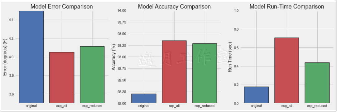
Where original represents old data, that is, the part with little data and few features; exp_all represents the complete new data; exp_reduced represents the part of the important feature dataset selected according to the 95% threshold.The result is clear that the more data and features there are, the better the effect will be, but the time efficiency will be reduced.
The decision-making of the final model needs to be judged by actual business applications, but the analysis must be in place.
9.3 Model Tuning
Previously, the main aspect of comparative analysis was data and characteristics, and there was another very important work waiting for you to do, that is, model parameter adjustment. At the end of the experiment, see how to adjust parameters for tree models.
Adjusting parameters is a necessary step in machine learning. Many methods and experiences are not specific to an algorithm, and basic general tasks can be used for reference.
Print first to see what parameters are available:
 1 import pandas as pd
 2 features = pd.read_csv('data/temps_extended.csv')
 3
 4 features = pd.get_dummies(features)
 5
 6 labels = features['actual']
 7 features = features.drop('actual', axis = 1)
 8
 9 feature_list = list(features.columns)
10
11 import numpy as np
12
13 features = np.array(features)
14 labels = np.array(labels)
15
16 from sklearn.model_selection import train_test_split
17
18 train_features, test_features, train_labels, test_labels = train_test_split(features, labels,
19                                                                             test_size = 0.25, random_state = 42)
20
21 print('Training Features Shape:', train_features.shape)
22 print('Training Labels Shape:', train_labels.shape)
23 print('Testing Features Shape:', test_features.shape)
24 print('Testing Labels Shape:', test_labels.shape)
25
26 print('{:0.1f} years of data in the training set'.format(train_features.shape[0] / 365.))
27 print('{:0.1f} years of data in the test set'.format(test_features.shape[0] / 365.))
28
29 important_feature_names = ['temp_1', 'average', 'ws_1', 'temp_2', 'friend', 'year']
30
31 important_indices = [feature_list.index(feature) for feature in important_feature_names]
32
33 important_train_features = train_features[:, important_indices]
34 important_test_features = test_features[:, important_indices]
35
36 print('Important train features shape:', important_train_features.shape)
37 print('Important test features shape:', important_test_features.shape)
38
39 train_features = important_train_features[:]
40 test_features = important_test_features[:]
41
42 feature_list = important_feature_names[:]
1 from sklearn.ensemble import RandomForestRegressor
2
3 rf = RandomForestRegressor(random_state = 42)
4
5 from pprint import pprint
6
7 # Print all parameters
8 pprint(rf.get_params())
The explanation of the parameters has been described in the Decision Tree algorithm. When using a toolkit to complete a task, it is best to first look at its API documentation, where the meaning of each parameter and its input numeric type are clear
https://scikit-learn.org/stable/modules/classes.html
When you need to find some instructions, you can press and hold the Ctrl+F key combination directly to search for keywords in your browser, for example, to find RandomForestRegressor, find its corresponding location and click inside.
This address bar you can put together directly.
When there is a large amount of data, it may be less direct to observe the results directly with the functions in the toolkit, or you can construct a simple input to observe the results yourself, make sure there are no errors, and then execute with the complete data.
9.3.1 Random parameter selection
There are a long way to adjust parameters. There are really too many possible combinations of parameters. Assuming there are five parameters to be determined and there are 10 candidate values for each parameter, how many possibilities are there (but not as simple as 5 by 10)?That's a big number. In actual business, because of the large amount of data and the relatively complex model, it takes a lot of time. It's good to finish the model once in a few hours.So how do you choose the parameters that are more appropriate?If you go through all the possible scenarios in turn, you're probably going to end up in the wilderness.
The first step is RandomizedSearchCV, a function that helps you continuously randomly select an appropriate set of parameters in the parameter space to model and evaluate the results after cross-validation.
Why choose randomly?One by one should be more reliable, but it really doesn't take time to walk through the search, and randomness becomes a strategy.It's like randomly testing all the possible parameters to find roughly feasible locations, and it feels a bit unreliable, but it's also helpless.All the parameter explanations required for this function are detailed in the API documentation and can be called directly after the model, data, and parameter spaces are prepared.
 1 from sklearn.model_selection import RandomizedSearchCV
 2
 3 # Number of trees built
 4 n_estimators = [int(x) for x in np.linspace(start = 200, stop = 2000, num = 10)]
 5 # Selection of Maximum Features
 6 max_features = ['auto', 'sqrt']
 7 # Maximum depth of tree
 8 max_depth = [int(x) for x in np.linspace(10, 20, num = 2)]
 9 max_depth.append(None)
10 # Number of samples required for minimum node splitting
11 min_samples_split = [2, 5, 10]
12 # Leaf node minimum number of samples, any split cannot make its child node number less than this value
13 min_samples_leaf = [1, 2, 4]
14 # Sample sampling method
15 bootstrap = [True, False]
16
17 # Random grid
18 random_grid = {'n_estimators': n_estimators,
19                'max_features': max_features,
20                'max_depth': max_depth,
21                'min_samples_split': min_samples_split,
22                'min_samples_leaf': min_samples_leaf,
23                'bootstrap': bootstrap}
In this task, only examples are given to illustrate that the candidate values for the selected parameters are not too many due to the length of the task.It is worth noting that the range of values for each parameter needs to be well controlled, because if the range of parameters is inappropriate, the final result will certainly not be good.You can adjust the appropriate parameter space by referencing some empirical values or continuously experimenting with the results.
Adjusting parameters is also an iterative process, which does not mean that the task of machine learning modeling is carried out from the beginning to the end. After the experimental results are confirmed, it is necessary to go back and compare different parameters and different preprocessing schemes repeatedly.
Explain the parameters commonly used in RandomizedSearchCV, API documentation gives detailed instructions, I suggest you develop the habit of consulting documentation.
- Estmator: RandomizedSearchCV is a general function that is not designed for random forests, so you need to specify what the selected algorithm model is.
- distributions: The candidate space for a parameter, and the required parameter distribution has been given in dictionary format in the code above.
- N_iter: The number of random combinations of parameters, such as n_iter=100, represents the next 100 random combinations of parameters to find the best one.
- scoring: the evaluation method by which to find the best combination of parameters.
- cv: cross-validation, as described earlier.
- verbose: the number of printed information, according to your needs.
- random_state: Random seeds, in order to make the results consistent and eliminate the interference of random components, are usually assigned a value, just use your own lucky number.
- N_jobs: Run this program with multiple threads. If 1, all will be used, but there may be a bit of a card.Even if n_jobs is set to 1, the program runs a little slowly, because to build a 100-time model to select parameters, with a 3-fold cross-validation, it's equivalent to 300 tasks.
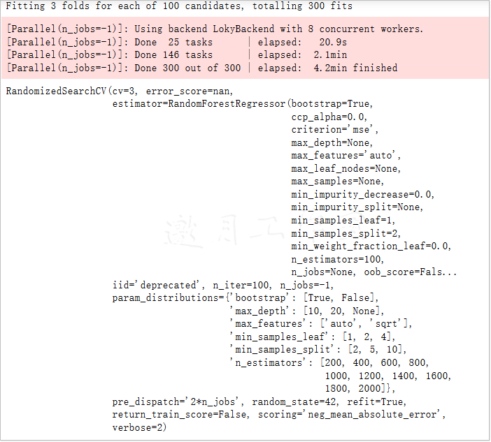
RandomizedSearch results show the time and the current number of times a task is executed. If the data is large and you need to wait for a while, simply understand the intermediate results. Finally, call rf_random.best_params_ directly to get the best set of parameters out of the 100 random selections:
1 # Randomly select the most appropriate combination of parameters
2 rf = RandomForestRegressor()
3
4 rf_random = RandomizedSearchCV(estimator=rf, param_distributions=random_grid,
5                               n_iter = 100, scoring='neg_mean_absolute_error',
6                               cv = 3, verbose=2, random_state=42, n_jobs=-1)
7
8 # Perform Find
9 rf_random.fit(train_features, train_labels)
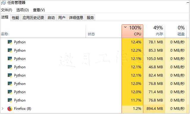
The running time mainly depends on that your CPU s are not hard enough.
1 rf_random.best_params_
{'n_estimators': 1400,
 'min_samples_split': 10,
 'min_samples_leaf': 4,
 'max_features': 'auto',
 'max_depth': 10,
 'bootstrap': True}
After 100 random selections, you can also get other experimental results, which are explained in the API documentation. This is not demonstrated here. Readers who like to do it can try it themselves.
Next, compare the results of random tuning with those of default parameters, all default parameters are explained in the API, such as n_estimators:integer,optional (default=10), which means that in the random forest model, the default number of trees to be built is 10.
In general, parameters have default values, not that you don't need them without giving them, but that you use their default values in your code.
Consistent with previous experiments, whether a comparative analysis is needed or an evaluation criterion is given first:
1 def evaluate(model, test_features, test_labels):
2     predictions = model.predict(test_features)
3     errors = abs(predictions - test_labels)
4     mape = 100 * np.mean(errors / test_labels)
5     accuracy = 100 - mape
6
7     print('Average Temperature Error.',np.mean(errors))
8     print('Accuracy = {:0.2f}%.'.format(accuracy))
1 base_model = RandomForestRegressor( random_state = 42)
2 base_model.fit(train_features, train_labels)
3 evaluate(base_model, test_features, test_labels)
Average temperature error. 3.829032846715329
Accuracy = 93.56%.
1 best_random = rf_random.best_estimator_
2 evaluate(best_random, test_features, test_labels)
Average temperature error. 3.7145380641444214
Accuracy = 93.73%.
From the above comparison experiments, we can see that the effect of the model has been improved a little, the original error is 3.83, and the error after adjusting parameters has decreased to 3.71.But is this the upper limit?Is there any room for progress?In the previous explanation, it was also mentioned that the random parameter selection is to find a general direction, but it is certainly not perfect, as if the police were arresting a criminal suspect, getting the general location first, then carpet search.
9.3.2 Network Parameter Search
Next, the next contestant, GridSearchCV(), will do the same thing as his name, doing a web search, that is, traversing one by one, without losing any possible combination of parameters.As mentioned before, walk through all the combinations, using the same method as RandomizedSearchCV(), but with different names.
https://scikit-learn.org/stable/modules/generated/sklearn.model_selection.GridSearchCV.html
 1 from sklearn.model_selection import GridSearchCV
 2
 3 # Web Search
 4 param_grid = {
 5     'bootstrap': [True],
 6     'max_depth': [8,10,12],
 7     'max_features': ['auto'],
 8     'min_samples_leaf': [2,3, 4, 5,6],
 9     'min_samples_split': [3, 5, 7],
10     'n_estimators': [800, 900, 1000, 1200]
11 }
12
13 # Select basic algorithm model
14 rf = RandomForestRegressor()
15
16 # Web Search
17 grid_search = GridSearchCV(estimator = rf, param_grid = param_grid,
18                            scoring = 'neg_mean_absolute_error', cv = 3,
19                            n_jobs = -1, verbose = 2)
20
21 # Perform Search
22 grid_search.fit(train_features, train_labels)
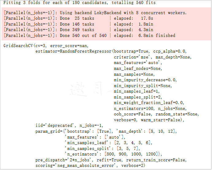
The CPU runs 100% long enough for you to warm up a cup of tea.

When using web search, it is worth noting that the choice of parameter space is based on experience or guess?There is already a set of results of random parameter selection, which is equivalent to the general direction already obtained in a large range of parameter space. The next network search should continue based on the previous experiment, using the results of random parameter selection as the basis for the next network search.This is equivalent to having a general area of activity for the criminal suspect (the best model parameters) at this point, and a carpet capture is to be launched.
When there is a large amount of data and it is not possible to directly adjust network search parameters, you may also consider alternating random and network search strategies to simplify the number of required comparative experiments.
After readjustment, the effect of the algorithm model has been improved a little. Although it is only a small step, adding each small step together is a big achievement.When using web search, if the parameter space is large, traverse too many times, usually not putting all the possibilities in it, but dividing them into different groups, like a catch job is hard to find all carpet, but it's also possible to divide them into several groups to stay at important intersections.
Next, let's look at another set of web search contestants, with slightly different emphasis on each set of candidate parameters:
1 grid_search.best_params_
{'bootstrap': True,
 'max_depth': 12,
 'max_features': 'auto',
 'min_samples_leaf': 6,
 'min_samples_split': 3,
 'n_estimators': 900}
1 best_grid = grid_search.best_estimator_
2 evaluate(best_grid, test_features, test_labels)
Average temperature error. 3.6813587581120273
Accuracy = 93.78%.
It looks like the second group of players is a little more powerful than the first, and after this toss (go to the coffee shop and come back to see the tea you just made).After ^^), you can list all the parameters that were selected, and the average temperature error is 3.66, which is equivalent to one of the best results:
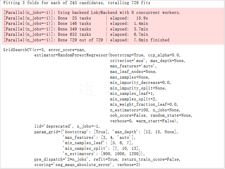
 1 param_grid = {
 2     'bootstrap': [True],
 3     'max_depth': [12, 15, None],
 4     'max_features': [3, 4,'auto'],
 5     'min_samples_leaf': [5, 6, 7],
 6     'min_samples_split': [7,10,13],
 7     'n_estimators': [900, 1000, 1200]
 8 }
 9
10 # Select algorithm model
11 rf = RandomForestRegressor()
12
13 # Keep searching
14 grid_search_ad = GridSearchCV(estimator = rf, param_grid = param_grid,
15                            scoring = 'neg_mean_absolute_error', cv = 3,
16                            n_jobs = -1, verbose = 2)
17
18 grid_search_ad.fit(train_features, train_labels)
1 grid_search_ad.best_params_
grid_search_ad.best_params_

{'bootstrap': True,
 'max_depth': 12,
 'max_features': 4,
 'min_samples_leaf': 7,
 'min_samples_split': 13,
 'n_estimators': 1200}
1 best_grid_ad = grid_search_ad.best_estimator_
2 evaluate(best_grid_ad, test_features, test_labels)
Average temperature error. 3.6642196127491156
Accuracy = 93.82%.
1 print('Final model parameters:\n')
2 pprint(best_grid_ad.get_params())
Final model parameters:

{'bootstrap': True,
 'ccp_alpha': 0.0,
 'criterion': 'mse',
 'max_depth': 12,
 'max_features': 4,
 'max_leaf_nodes': None,
 'max_samples': None,
 'min_impurity_decrease': 0.0,
 'min_impurity_split': None,
 'min_samples_leaf': 7,
 'min_samples_split': 13,
 'min_weight_fraction_leaf': 0.0,
 'n_estimators': 1200,
 'n_jobs': None,
 'oob_score': False,
 'random_state': None,
 'verbose': 0,
 'warm_start': False}
In the above output results, not only the parameters that have just been adjusted, but also the parameters using default values are displayed to facilitate analysis, and finally summarize the tuning tasks in machine learning.
- 1. Parametric space is important because it can have a decisive impact on the results, so before starting a task, you need to select a roughly appropriate interval that can refer to some of the experience values from the same task paper.
- 2. Random searches are relatively time-saving, especially at the beginning of a task, when you don't know where the parameters are and the results may be better, you can set the parameter interval a little larger and use random methods to determine a general location.
- 3. Web search is equivalent to carpet search and needs to traverse every possible combination in the parameter space, which is slower and can be used with random search.
- 4. There are many ways to adjust parameters, such as Bayesian optimization, which is still interesting. To briefly tell you, think about the previous ways of adjusting parameters, whether each of them is conducted independently and will not have any impact on the subsequent results?The basic idea of Bayesian optimization is that each optimization is constantly accumulating experience so that you can slowly get where the final solution should be, which is equivalent to the effect of the previous step on the future. If you are interested in Bayesian optimization, you can refer to the Hyperopt toolkit, which is very easy to use: https://pypi.org/project/hyperopt/ This is a reference: https://www.jianshu.com/p/35eed1567463
The disturbing thing about this installation is that it forces networkX to be reduced from 2.4 to 2.2. What is the anti-heavenly logic?Be careful!
pip install hyperopt
/*
Looking in indexes: https://pypi.tuna.tsinghua.edu.cn/simple
...
Successfully built networkx
Installing collected packages: cloudpickle, networkx, tqdm, hyperopt
  Attempting uninstall: networkx
    Found existing installation: networkx 2.4
    Uninstalling networkx-2.4:
      Successfully uninstalled networkx-2.4
Successfully installed cloudpickle-1.3.0 hyperopt-0.2.3 networkx-2.2 tqdm-4.45.0
Project summary:
In the actual warfare task of temperature prediction based on random forest, the whole module is divided into three parts to interpret. First, the basic random forest model construction and visualization methods are explained.Then, by comparing the impact of the amount of data and the number of features on the results, it is recommended that as many data features and processing schemes as possible be selected at the beginning of the task to facilitate subsequent comparative experiments and analysis.Finally, the parameter adjustment process is also an essential part of machine learning, and the appropriate strategy can be selected according to business needs and actual data volume.
Chapter 9 is complete.