python data analysis personal study reading notes - Catalog Index
Chapter 4 statistics and linear algebra
Statistics and linear algebra lay the foundation for exploratory data analysis. Both descriptive and inferential statistical methods are helpful to obtain insights and inferences from the original data. For example, after calculating the arithmetic mean and standard deviation of the variable through the data, and then deriving the value range and expected value of the variable, we can use the statistical test to evaluate the reliability of the conclusion.
Linear algebra focuses on solving linear equations, and the linaling package of NumPy and SciPy can help us solve this problem easily. Linear algebra is widely used, for example, it is necessary to fit data by model. In addition, this chapter introduces several other NumPy and SciPy packages, including random number generation and Masked arrays.
This chapter deals with the following topics.
- Using NumPy to deal with simple descriptive statistics
- Linear algebra operation with NumPy
- Using NumPy to find eigenvalues and eigenvectors
- NumPy random number
- Create NumPy Masked arrays
4.1 simple descriptive statistical calculation with NumPy
In this book, we will try to use various data sets that can be obtained through open channels. However, the theme of these data may not be exactly what the readers are interested in. In addition, although each data set has its own characteristics, the techniques introduced in this book are universal, so they are also applicable to everyone's fields. In this chapter, we load the dataset from the statsmodels library into the NumPy array for data analysis.
Mauna Loa CO2 measurement data is the first data set of the statsmodels library we use. The following code loads the dataset and gives basic descriptive statistics.
 1 import numpy as np
 2 from scipy.stats import scoreatpercentile
 3 import pandas as pd
 4
 5 data = pd.read_csv("co2.csv", index_col=0, parse_dates=True)
 6
 7 co2 = np.array(data.co2)
 8
 9 print("The statistical valus for amounts of co2 in atmosphere : \n")
10 print("Max method : ", co2.max())
11 print("Max function : ", np.max(co2))
12
13 print("Min method : ", co2.min())
14 print("Min function : ", np.min(co2))
15
16 print("Mean method : ", co2.mean())
17 print("Mean function : ", np.mean(co2))
18
19 print("Std method : ", co2.std())
20 print("Std function : ", np.std(co2))
21
22 print("Median : ", np.median(co2))
23 print("Score at percentile 50 : ", scoreatpercentile(co2, 50))
The above code calculates the average, median, maximum, minimum, and standard deviation of the NumPy array.
Tips: if these terms don't sound familiar, take the time to go to Wikipedia or other places to learn about them. In the foreword, the book assumes that the reader is familiar with basic mathematical and statistical concepts.
The data used here are from the statsmodels package, which are the atmospheric CO2 values observed by Mauna Loa Observatory in Hawaii.
Now, let's look at the specific code.
(1) first, use the import statement to load the relevant modules of Python package, as follows.
1 import numpy as np
2 from scipy.stats import scoreatpercentile
3 import pandas as pd
(2) then, call the following function to load the data.
1 data = pd.read_csv("co2.csv", index_col=0, parse_dates=True)
2
3 co2 = np.array(data.co2)
The data in the above code will be copied to the NumPy array CO2, which is used to store the CO2 observations in the atmosphere.
(3) the maximum value of the array can be obtained through the method of ndarray or other NumPy functions, and the minimum value, average value and standard deviation are the same. The following code will display various statistical indicators.
 1 print("The statistical valus for amounts of co2 in atmosphere : \n")
 2 print("Max method : ", co2.max())
 3 print("Max function : ", np.max(co2))
 4
 5 print("Min method : ", co2.min())
 6 print("Min function : ", np.min(co2))
 7
 8 print("Mean method : ", co2.mean())
 9 print("Mean function : ", np.mean(co2))
10
11 print("Std method : ", co2.std())
12 print("Std function : ", np.std(co2))
The output is as follows.
Max method :  366.84
Max function :  366.84
Min method :  313.18
Min function :  313.18
Mean method :  337.0535256410256
Mean function :  337.0535256410256
Std method :  14.950221626197369
Std function :  14.950221626197369
(4) the median can be obtained by using the function of NumPy or SciPy. The following code will calculate the 50th percentile of the data.
1 print("Median : ", np.median(co2))
2 print("Score at percentile 50 : ", scoreatpercentile(co2, 50))
Here is the output.
Median :  335.17
Score at percentile 50 :  335.17
4.2 linear algebra operation with NumPy
Linear algebra is an important branch of mathematics. For example, we can use linear algebra to solve linear regression problems. The subroutine package numpy.linalg provides many linear algebra routines, which can be used to calculate the inverse or eigenvalue of a matrix, solve linear equations or calculate determinants. For NumPy, matrices can be represented by a subclass of ndarray.
4.2.1 finding the inverse of matrix with NumPy
In linear algebra, suppose a is a square matrix or invertible matrix. If there is a matrix A-1, it satisfies the condition that the matrix A-1 is equal to the unit matrix I when multiplied by the original matrix A, then the matrix A-1 is the inverse of A. the corresponding mathematical equations are as follows.
A A-1 = I
The inv() function in the subroutine numpy. Linaling is used to find the inverse of matrix. Here is an example to illustrate the specific steps as follows.
(1) using the mat() function to create an example matrix.
A = np.mat("2 4 6;4 2 6;10 -4 18")
print("A\n", A)
Matrix A is as follows.
A
 [[ 2  4  6]
 [ 4  2  6]
 [10 -4 18]]
(2) find the inverse of matrix. Now you can use the inv() subroutine to calculate the inverse matrix.
1 inverse = np.linalg.inv(A)
2 print("inverse of A\n", inverse)
The inverse matrix is shown below.
inverse of A
 [[-0.41666667  0.66666667 -0.08333333]
 [ 0.08333333  0.16666667 -0.08333333]
 [ 0.25       -0.33333333  0.08333333]]
Tips: if the matrix is singular or non square, we will get LinAlgError message. If we like, we can also verify the calculation result manually. The pinv() function in NumPy library can be used to find the pseudo inverse matrix, which is suitable for any matrix, including non square matrix.
(3) use multiplication to check.
Next, we multiply the calculation result of inv() function by the original matrix to check whether the calculation result is correct.
1 print("Check\n", A * inverse)
As we expected, we did get a unit matrix (provided, of course, that some small errors are ignored).
Check
 [[ 1.00000000e+00  1.11022302e-16 -2.77555756e-17]
 [-2.22044605e-16  1.00000000e+00 -2.77555756e-17]
 [-8.88178420e-16  1.22124533e-15  1.00000000e+00]]
If we subtract the unit matrix of 3 × 3 from the above calculation result, we will get the error in the process of inversion.
1 print("Error\n", A * inverse - np.eye(3))
Generally speaking, these errors are usually ignored, but in some cases, small errors may also lead to adverse consequences.
Error
 [[-1.11022302e-16  1.11022302e-16 -2.77555756e-17]
 [-2.22044605e-16  4.44089210e-16 -2.77555756e-17]
 [-8.88178420e-16  1.22124533e-15 -2.22044605e-16]]
In this case, we need to use more precise data types, or more advanced algorithms. Previously, we used the inv() routine of the numpy.linaling subroutine to calculate the inverse of the matrix. Next, we use matrix multiplication to verify whether the inverse matrix meets our requirements.
1 import numpy as np
2 A = np.mat("2 4 6;4 2 6;10 -4 18")
3 print "A\n", A
4
5 inverse = np.linalg.inv(A)
6 print("inverse of A\n", inverse)
7
8 print("Check\n", A * inverse)
9 print("Error\n", A * inverse - np.eye(3))
4.2.2 solving linear equations with NumPy
Matrix can transform one vector into another in A linear way, so from the point of view of numerical calculation, this operation corresponds to A system of linear equations. The solve() subroutine in numpy.lingcan solve linear equations in the form of Ax = b, where A is A matrix, b is A one-dimensional or two-dimensional array, and x is an unknown quantity. Next, we show how to use the dot() function to calculate the dot product of two floating-point arrays.
Here is an example to illustrate the process of solving linear equations. The specific steps are as follows.
(1) first create matrix A and array b.
The code for creating matrix A and array b is as follows.
1 A = np.mat("1 -2 1;0 2 -8;-4 5 9")
2 print("A\n", A)
3
4 b = np.array([0, 8, -9])
5 print("b\n", b)
Matrix A and array (vector) b are defined as follows.
A
 [[ 1 -2  1]
 [ 0  2 -8]
 [-4  5  9]]
b
 [ 0  8 -9]
(2) call the solve() function.
(3) next, we use the solve() function to solve the linear equations.
1 x = np.linalg.solve(A, b)
2 print("Solution", x)
The solutions of linear equations are as follows.
Solution [29. 16. 3.]
(4) we use dot() function to check.
We use the dot() function to check whether the solution is correct.
1 print("Check\n", np.dot(A , x))
The result was as expected.
Check[[ 0. 8. -9.]]
Previously, we solved the linear equations by the solve() function in the linaling subroutine of NumPy, and checked the results by using the dot() function. Let's put these codes together.
 1 import numpy as np
 2
 3 A = np.mat("1 -2 1;0 2 -8;-4 5 9")
 4 print("A\n", A)
 5
 6 b = np.array([0, 8, -9])
 7 print("b\n", b)
 8
 9 x = np.linalg.solve(A, b)
10 print("Solution", x)
11
12 print("Check\n", np.dot(A , x))
13
14
4.3 calculation of eigenvalues and eigenvectors with NumPy
Eigenvalues are scalar solutions of equation Ax=ax, where A is A two-dimensional matrix and x is A one-dimensional vector. The eigenvector is actually the vector representing the eigenvalue.
Tips: eigenvalues and eigenvectors are basic mathematical concepts and are often used in some important algorithms, such as principal component analysis (PCA) algorithm. PCA can greatly simplify the analysis process of large-scale data sets.
When calculating eigenvalues, we can turn to the eigvals() subroutine provided by the numpy. Linaling package. The return value of function eig() is a tuple, and its elements are eigenvalues and eigenvectors.
We can use the eigvals() and eig() functions of the subroutine numpy.linalg to get the eigenvalues and eigenvectors of the matrix, and use the dot() function to check the results.
 1 import numpy as np
 2 A = np.mat("3 -2;1 0")
 3 print("A\n", A)
 4
 5 print("Eigenvalues", np.linalg.eigvals(A))
 6
 7 eigenvalues, eigenvectors = np.linalg.eig(A)
 8 print("First tuple of eig", eigenvalues)
 9 print("Second tuple of eig\n", eigenvectors)
10
11 for i in range(len(eigenvalues)):
12    print("Left", np.dot(A, eigenvectors[:,i]))
13    print("Right", eigenvalues[i] * eigenvectors[:,i])
Let's calculate the eigenvalues of a matrix.
(1) we create a matrix.
(2) the following code will create a matrix.
1 A = np.mat("3 -2;1 0")
2 print("A\n", A)
The following matrix is the one you just created.
A
 [[ 3 -2]
 [ 1  0]]
(2) using the eig() function to calculate the eigenvalue.
At this point, we can use the eig() subroutine.
1 Print("Eigenvalues", np.linalg.eigvals(A))
The eigenvalues of the matrix are as follows.
Eigenvalues [2. 1.]
(3) using the eig() function to get the eigenvalues and eigenvectors.
Using the eig() function, we can get the eigenvalues and eigenvectors. Note that the function returns a tuple, its first element is the eigenvalue, and its second element is the corresponding eigenvectors, arranged in a column oriented manner.
1 eigenvalues, eigenvectors = np.linalg.eig(A)
2 print("First tuple of eig", eigenvalues)
3 print("Second tuple of eig\n", eigenvectors)
The eigenvalues and eigenvectors are as follows.
First tuple of eig [2. 1.]
Second tuple of eig
 [[0.89442719 0.70710678]
 [0.4472136  0.70710678]]
(4) checking calculation results.
By calculating the values on both sides of the eigenvalue equation Ax = ax with the dot() function, we can check the results.
1 for i in range(len(eigenvalues)):
2    print("Left", np.dot(A, eigenvectors[:,i]))
3    print("Right", eigenvalues[i] * eigenvectors[:,i])
The output is as follows.
Left [[1.78885438]
 [0.89442719]]
Right [[1.78885438]
 [0.89442719]]
Left [[0.70710678]
 [0.70710678]]
Right [[0.70710678]
 [0.70710678]]
4.4 numpy random number
Random number is often used in Monte Carlo method, random integral and so on. However, the real random number is very difficult to obtain. In practice, the pseudo-random number is used. In most cases, pseudo-random numbers are enough to meet our needs. Of course, except for some special cases, such as high-precision simulation experiments. For NumPy, functions related to random numbers are in the random subroutine.
Tip: the random number generator of NumPy core is based on Mason rotation algorithm.
We can generate both continuous and discontinuous random numbers. The distribution function has an optional size parameter that tells NumPy how many numbers to create. We can use integer or tuple to assign a value to this parameter. Then we will get an array of corresponding shape, whose value is filled by random number. The discrete distribution includes geometric distribution, hypergeometric distribution and binomial distribution. Continuous distribution includes normal distribution and lognormal distribution.
4.4.1 game with binomial distribution
Binomial distribution is used to simulate the number of successful experiments in the whole number of independent experiments, and the chances of success in each experiment are certain.
Suppose we were in the 17th century, betting on eight pieces of money. It was popular to play with nine coins. If there are less than five coins with heads up, we will lose an 8-cent; otherwise, we will win an 8-cent. Now, let's start to simulate the game, assuming we have 1000 coins in hand as initial funding. We will use the binomial() function provided by the random module for simulation.
Tips: see ch-04.ipynb in the code package of this book for the complete code.
 1 import numpy as np
 2 from matplotlib.pyplot import plot, show
 3
 4 cash = np.zeros(10000)
 5 cash[0] = 1000
 6 outcome = np.random.binomial(9, 0.5, size=len(cash))
 7
 8 for i in range(1, len(cash)):
 9
10    if outcome[i] < 5:
11       cash[i] = cash[i - 1] - 1
12    elif outcome[i] < 10:
13       cash[i] = cash[i - 1] + 1
14    else:
15       raise AssertionError("Unexpected outcome " + outcome)
16
17 print(outcome.min(), outcome.max())
18
19 plot(np.arange(len(cash)), cash)
20 show()
If you want to understand the binary () function, see the following steps.
(1) we use the binomial() function.
We initialize the array to zero, which means the cash balance is zero. Call the binomial() function and set the size parameter to 10000, which means we have to flip 10000 coins.
1 cash = np.zeros(10000)
2 cash[0] = 1000
3 outcome = np.random.binomial(9, 0.5, size=len(cash))
(2) update the cash balance.
We use the result of flipping Zheng coins to update the cash array and display the maximum and minimum values in the output array, as long as there is no rare abnormal value.
 1 for i in range(1, len(cash)):
 2
 3    if outcome[i] < 5:
 4       cash[i] = cash[i - 1] - 1
 5    elif outcome[i] < 10:
 6       cash[i] = cash[i - 1] + 1
 7    else:
 8       raise AssertionError("Unexpected outcome " + outcome)
 9
10 print(outcome.min(), outcome.max())
As expected, the value is 0-9.
0 9
(3) draw the image of cash array with matplotlib.
1 Plot(np.arange(len(cash)), cash)
2 Show()
As can be seen from Figure 4-2, the curve of cash balance is similar to random walk (i.e. not according to fixed mode, but random walk).
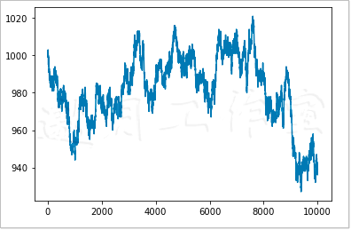
Of course, every time we execute program code, we get a different random walk. If you want to always get the same result, you need to give a seed value to the binomial() function in NumPy's random number subpackage.
4.4.2 sampling of normal distribution
Continuous distribution is modeled by probability density function (PDF). The probability of an event occurring in a specific interval can be calculated by integral operation of probability density function. NumPy's random module provides many functions representing continuous distribution, such as beta, chisquare, exponential, F, gamma, gumbel, laplace, lognormal, logistic, multivariate_normal, noncentral_chinese, noncentral_f, normal, etc.
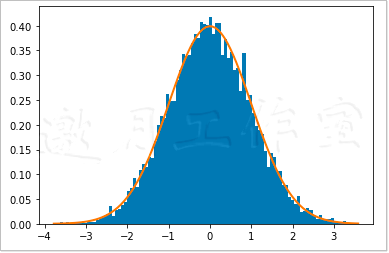
By using the normal() function in NumPy's random subroutine, the normal distribution can be shown in an intuitive form. Here are the bell curves and bar graphs of randomly generated values.
 1 import numpy as np
 2 import matplotlib.pyplot as plt
 3
 4 N=10000
 5
 6 normal_values = np.random.normal(size=N)
 7 #dummy, bins, dummy = plt.hist(normal_values, int(np.sqrt(N)), normed =True, lw=1)
 8 #normed: Boolean values. It is not recommended by the government. It is recommended to use it instead density Parameters.
 9 dummy, bins, dummy = plt.hist(normal_values, int(np.sqrt(N)), density =True, lw=1)
10 sigma = 1
11 mu = 0
12 plt.plot(bins, 1/(sigma * np.sqrt(2 * np.pi)) * np.exp( - (bins - mu)**2 / (2 * sigma**2) ),lw=2)
13 plt.show()
Random numbers can be generated according to the requirements of normal distribution, and their distribution can be displayed by bar graph. If you want to draw a normal distribution, follow these steps.
(1) generate values.
With the normal() function provided by NumPy's random subroutine, you can create a specified number of random numbers.
1 N=10000
2
3 normal_values = np.random.normal(size=N)
(2) draw bar chart and theoretical PDF.
Next, use matplotlib to draw bar graphs and theoretical PDF s, where the center value is 0 and the standard deviation is 1.
1 #dummy, bins, dummy = plt.hist(normal_values, int(np.sqrt(N)), normed =True, lw=1)
2 #normed: Boolean values. It is not recommended by the government. It is recommended to use it instead density Parameters.
3 dummy, bins, dummy = plt.hist(normal_values, int(np.sqrt(N)), density =True, lw=1)
4 sigma = 1
5 mu = 0
6 plt.plot(bins, 1/(sigma * np.sqrt(2 * np.pi)) * np.exp( - (bins - mu)**2 / (2 * sigma**2) ),lw=2)
7 plt.show()
Figure 4-3 shows the famous bell curve.
4.4.3 normal inspection with SciPy
Normal distribution is widely used in the field of science and statistics. According to the central limit theorem, with the increase of the number of independent random samples, they tend to normal distribution. The properties of normal distribution are well known, and it is also very easy to use. However, it needs to meet many necessary conditions, such as the number of data points is large enough, and the data points must be independent of each other. At work, we need to develop a good habit of checking whether the data conforms to the normal distribution. There are many methods of normal test, some of which have been implemented in the skip.stats package. These tests are used in this section. The samples are influenza trend data from Google website. Here we have simplified the original document, leaving only two columns of date and data from Argentina. Here is the routine.
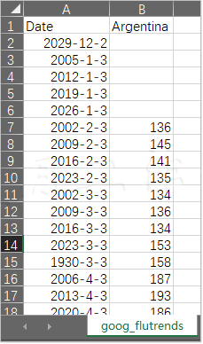
These data can be found in the Google flutrends.csv file in the code package of this book. As before, we also sample these data according to the normal distribution here. The size of the obtained array is the same as that of the flu trend array. If it passes the normal test successfully, it will be taken as the golden standard. The code here is taken from the ch-04.ipynb file in the code package.
 1 import numpy as np
 2 from scipy.stats import shapiro
 3 from scipy.stats import anderson
 4 from scipy.stats import normaltest
 5
 6 flutrends = np.loadtxt("goog_flutrends.csv", delimiter=',', usecols=(1,), skiprows=1, converters = {1: lambda s: float(s or 0)}, unpack=True)
 7 N = len(flutrends)
 8 normal_values = np.random.normal(size=N)
 9 zero_values = np.zeros(N)
10
11 print("Normal Values Shapiro", shapiro(normal_values))
12 #print("Zeroes Shapiro", shapiro(zero_values))
13 print("Flu Shapiro", shapiro(flutrends))
14
15 print("Normal Values Anderson", anderson(normal_values))
16 #print("Zeroes Anderson", anderson(zero_values))
17 print("Flu Anderson", anderson(flutrends))
18
19 print("Normal Values normaltest", normaltest(normal_values))
20 #print("Zeroes normaltest", normaltest(zero_values))
21 print("Flu normaltest", normaltest(flutrends))
As a negative example, the array used below is the same size as the zero filled array mentioned earlier. In fact, this kind of data may be encountered when dealing with some small probability events (such as the outbreak of a world epidemic).
In this data file, some cells are empty. Of course, this kind of problem often occurs, so we must get used to cleaning the data first. Let's assume that the correct value is zero. Let's use a converter to fill in these zero values.
See line 6 above
Shapiro Wilke test can be used to test the normality. The corresponding SciPy function returns a tuple, where the first element is a test statistic and the second value is a p value. Note that this zero filled array raises a warning. In fact, the three functions used in this example do have difficulties in handling this array, and they also raise warnings. Here are the results.
Normal Values Shapiro (0.9963182806968689, 0.18643833696842194)
Flu Shapiro (0.9351990818977356, 2.2945883254311397e-15)
The p value obtained here is similar to the result of the third test later in this example. The analysis results are basically the same.
Anderson darling test can be used to test normal distribution and other distributions, such as exponential distribution, logarithmic distribution and Gumbel distribution. The relevant SciPy function involves a test statistic and an array that holds the thresholds corresponding to percentages of 15, 10, 5, 2.5, and 1. If the statistic is larger than the critical value of significance level, we can conclude that it is not normal. We will get the following values.
Normal Values Anderson AndersonResult(statistic=0.5299815280259281, critical_values=array([0.572, 0.652, 0.782, 0.912, 1.085]), significance_level=array([15. , 10. ,  5. ,  2.5,  1. ]))
Flu Anderson AndersonResult(statistic=8.258614154768793, critical_values=array([0.572, 0.652, 0.782, 0.912, 1.085]), significance_level=array([15. , 10. ,  5. ,  2.5,  1. ]))
We have nothing to say about this zero filled array, because the statistics returned are not a number at all. As we expected, this gold standard array is normal. However, this statistic returned by influenza trend data is larger than all relevant thresholds, so we can be sure that it does not conform to the normal distribution. Of the three test functions, this one seems to be the easiest to use.
SciPy's normal test() function also implements D'Agostino and Pearson tests. The tuple returned by this function, like shapiro(), also includes a statistic and P value. The p-value here is the two-sided chi squared probability. The chi square distribution is another famous distribution. This test itself is based on the z-fraction of the skewness and kurtosis tests. The skewness coefficient is used to express the degree of symmetry of the distribution. Because the normal distribution is symmetric, the skewness coefficient is zero. Kurtosis coefficient describes the shape of the distribution (peak, fat tail). The kurtosis coefficient of this normal distribution is 3, and the coefficient of excess kurtosis is 0. The following are the values obtained in this inspection.
Normal Values normaltest NormaltestResult(statistic=3.8850841487225543, pvalue=0.14333910757583423)
Flu normaltest NormaltestResult(statistic=99.64373336356954, pvalue=2.304826411536872e-22)
Because it deals with the probability of the p value, the larger it is, the better, it's better to be close to 1. For this zero filled array, you get very strange results. However, because we have been prompted, the result is not credible for this particular array. In addition, if P is equal to or greater than 0.5, it is considered to be normal. For the gold standard array, we will get a smaller value, which means we need to do more observation. As an assignment, please practice it yourself.
4.5 creating masked NumPy arrays
Data is often messy, and contains blank items or characters that cannot be processed. Fortunately, mask array can ignore incomplete or invalid data points. The mask array provided by the Numpy.ma subroutine belongs to the darray, with a mask. In this section, we use Lena Soderberg's photos as the data source, and assume that some data has been destroyed. The following is the complete code for handling mask array, which is taken from the ch – 04.ipynb file in the code package of this book.
 1 import numpy
 2 import scipy
 3 import matplotlib.pyplot as plt
 4
 5 face = scipy.misc.face()
 6
 7 random_mask = numpy.random.randint(0, 2, size=face.shape)
 8
 9 plt.subplot(221)
10 plt.title("Original")
11 plt.imshow(face)
12 plt.axis('off')
13
14 masked_array = numpy.ma.array(face, mask=random_mask)
15
16 plt.subplot(222)
17 plt.title("Masked")
18 plt.imshow(masked_array)
19 plt.axis('off')
20
21 plt.subplot(223)
22 plt.title("Log")
23 plt.imshow(numpy.ma.log(face).astype("float32"))
24 plt.axis('off')
25
26
27 plt.subplot(224)
28 plt.title("Log Masked")
29 plt.imshow(numpy.ma.log(masked_array).astype("float32"))
30 plt.axis('off')
31
32 plt.show()
Finally, we will show the original map, its pair value, mask array and its pair value.
(1) create a mask.
In order to get a mask array, a mask must be specified. Next, a random mask will be generated. The value of this mask is not 0, i.e. 1.
1 Random_mask = numpy.random.randint(0, 2, size=face.shape)
(2) create a mask array.
Next apply the mask to create a masked array.
1 Masked_array = numpy.ma.array(face, mask=random_mask)
We get Figure 4-4.
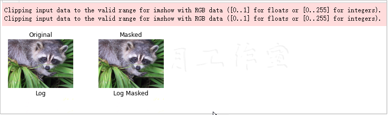
We attach a random mask to the NumPy array so that the data corresponding to the mask is ignored. The Numpy.ma subroutine provides all kinds of functions needed to process masked arrays. Here we only show how to generate masked arrays.
4.6 ignore negative and extreme values
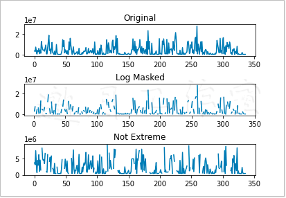
Masked arrays are very useful when you want to ignore negative values, such as logarithm of array values. In addition, masked arrays are also used to eliminate outliers. This work is based on the upper and lower limits of extremum. Here we take the salary data from MLB players as an example to illustrate the application of these technologies. After editing, this data only keeps the name and salary of the contestants, and the results are put in the MLB2008.csv file, which can be found in the code package of this book.
For the complete script, see the ch-04.ipynb file in the code package of this book.
 1 import numpy as np
 2 from datetime import date
 3 import sys
 4 import matplotlib.pyplot as plt
 5
 6 salary = np.loadtxt("MLB2008.csv", delimiter=',', usecols=(1,), skiprows=1, unpack=True)
 7 triples = np.arange(0, len(salary), 3)
 8 print("Triples", triples[:10], "...")
 9
10 signs = np.ones(len(salary))
11 print("Signs", signs[:10], "...")
12
13 signs[triples] = -1
14 print("Signs", signs[:10], "...")
15
16 ma_log = np.ma.log(salary * signs)
17 print("Masked logs", ma_log[:10], "...")
18
19 dev = salary.std()
20 avg = salary.mean()
21 inside = np.ma.masked_outside(salary, avg - dev, avg + dev)
22 print("Inside", inside[:10], "...")
23
24 plt.subplot(311)
25 plt.title("Original")
26 plt.plot(salary)
27
28 plt.subplot(312)
29 plt.title("Log Masked")
30 plt.plot(np.exp(ma_log))
31
32 plt.subplot(313)
33 plt.title("Not Extreme")
34 plt.plot(inside)
35
36 plt.subplots_adjust(hspace=.9)
37
38 plt.show()
The following is a description of the above command.
(1) logarithm of negative number
We can logarithm an array with negative numbers. First, create an array to store the array that can be divided by 3.
1 triples = np.arange(0, len(salary), 3)
2 print("Triples", triples[:10], "...")
Then an array with all element values of 1 and the size equal to the salary data array is generated.
1 signs = np.ones(len(salary))
2 print("Signs", signs[:10], "...")
With the help of the techniques learned in Chapter 2, you can reverse the value of an array element whose subscript is a multiple of 3.
1 signs[triples] = -1
2 print("Signs", signs[:10], "...")
Finally, we can get logarithm of this array.
1 ma_log = np.ma.log(salary * signs)
2 print("Masked logs", ma_log[:10], "...")
The corresponding salary data is shown below (note that some of the values here are NaN).
Triples [ 0  3  6  9 12 15 18 21 24 27] ...
Signs [1. 1. 1. 1. 1. 1. 1. 1. 1. 1.] ...
Signs [-1.  1.  1. -1.  1.  1. -1.  1.  1. -1.] ...
Masked logs [-- 14.970818190308929 15.830413578506539 -- 13.458835614025542
 15.319587954740548 -- 15.648092021712584 13.864300722133706 --] ...
(2) ignore extreme value
It is stipulated here that the so-called outliers are those values below one standard deviation of the average or above one standard deviation of the average. According to the above definition, the following code can be used to mask extreme points.
1 dev = salary.std()
2 avg = salary.mean()
3 inside = np.ma.masked_outside(salary, avg - dev, avg + dev)
4 print("Inside", inside[:10], "...")
The following code will show the first 10 elements.
Inside [3750000.0 3175000.0 7500000.0 3000000.0 700000.0 4500000.0 3000000.0
 6250000.0 1050000.0 4600000.0] ...
Next, draw the original salary data, logarithmic data and power recovery data respectively, and finally the data after applying the mask based on standard deviation.
See Figure 4-5 for details.
Functions in the Numpy.ma subpackage can mask elements in an array that are considered invalid, such as negative elements that cannot apply the log() and sqrt() functions. The masked value is similar to the NULL value in the relational database and programming. When calculating the masked value, it is given a masked value.
4.7 summary
In this chapter, we have studied various NumPy and SciPy sub libraries and reviewed the contents of linear algebra, statistics, continuous and discrete distribution, mask array and random number.
More techniques will be introduced in Chapter 5, although some may think that those jobs are not data analysis. In fact, we need to pay attention to everything that can be related to data analysis. Usually, when we do data analysis, we don't work in a fully staffed team, so no one will retrieve and store data for us. However, if you want to smoothly complete the data analysis process, these works are indispensable, so Chapter 5 will give a detailed description of these works.
The end of Chapter 4.
python data analysis personal study reading notes - Catalog Index
Official download of source code:
https://www.ptpress.com.cn/shopping/buy?bookId=bae24ecb-a1a1-41c7-be7c-d913b163c111
You need to log in and download it for free.