Machine vision is a branch of artificial intelligence which is developing rapidly. In short, machine vision is to use machines instead of human eyes to measure and judge. It is a comprehensive technology, including image processing, mechanical engineering technology, control, electrical lighting, optical imaging, sensors, analog and digital video technology, computer software and hardware technology (image enhancement and analysis algorithm, image card, I/O card, etc.).
. Python is a convenient high-level programming language with a small amount of code. OpenCV is a cross platform computer vision library licensed and distributed by BSD, which can run on Linux, Windows, Android and Mac OS operating systems. It is lightweight and efficient - it is composed of a series of C functions and a small number of C + + classes. At the same time, it provides interfaces of python, Ruby, MATLAB and other languages, and realizes many general algorithms in image processing and computer vision.
1: Edge extraction
In machine vision, a very basic operation is image processing, and in image processing, a very important knowledge is edge extraction. Edge extraction, exponential word image processing, for the image outline of a processing. For the boundary, where the gray value changes violently, it is defined as the edge. That is to say, inflection point refers to the point where the function changes concave convex. Associated with the derivative of high number, the edge of a given object is extracted. However, it is very convenient to use python+opencv for edge extraction.
The steps are as follows:
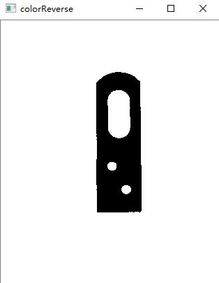
1. Threshold segmentation and color reversal of image
first, you need to create a new python file, import the cv2 Library (OpenCV2's python Library), and display a picture. The code is:
import cv2

# Read the initial.bmp file in this relative path
image = cv2.imread ("initial.bmp")
# Display the image corresponding to the image in the image window
cv2.imshow('initial',image)
# waitKey keeps the window static until the user presses a key
cv2.waitKey(0)
# The threshold value of image segmentation is set to 80, and the binary gray-scale image is obtained
ret,image1 = cv2.threshold(image,80,255,cv2.THRESH_BINARY)
cv2.imshow('grayscale',image1)
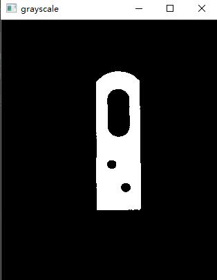
image2 = image1.copy()		# Copy pictures
for i in range(0,image1.shape[0]):	#image.shape represents the size and channel information of the image (height, width, channel)
for j in range(0,image1.shape[1]):
	image2[i,j]= 255 - image1[i,j]
cv2.imshow('colorReverse',image2)
2. Edge extraction
. The code is as follows:
# Edge extraction
img = cv2.cvtColor(image2,cv2.COLOR_BGR2GRAY)
canny_img_one = cv2.Canny(img,300,150)
canny_img_two = canny_img_one.copy()	# Copy pictures
for i in range(0,canny_img_one.shape[0]):	#image.shape represents the size and channel information of the image (height, width, channel)
	for j in range(0,canny_img_one.shape[1]):
		canny_img_two[i,j]= 255 - canny_img_one[i,j]
cv2.imshow('edge',canny_img_two)
finally, we can get an edge extracted figure, as follows: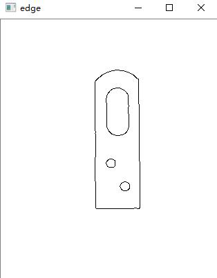
2: Image filtering
image filtering, that is, to suppress the noise of the target image under the condition of preserving the details of the image as much as possible, is an indispensable operation in image preprocessing. The quality of its processing effect will directly affect the effectiveness and reliability of subsequent image processing and analysis.
Noise is a kind of pollution caused by the imperfection of imaging system, transmission medium and recording equipment, during the formation, transmission and recording of digital image or in some links of image processing when the input image object is not as expected.
However, there are many filtering methods for image filtering. The filtering methods used in this experiment are mean filtering, median filtering, Gaussian filtering and Gaussian edge detection.
.
.
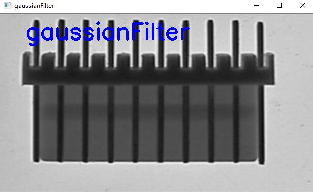
. Gaussian filtering is the process of weighted average of the whole image. The value of each pixel is obtained by weighted average of itself and other pixel values in the neighborhood.
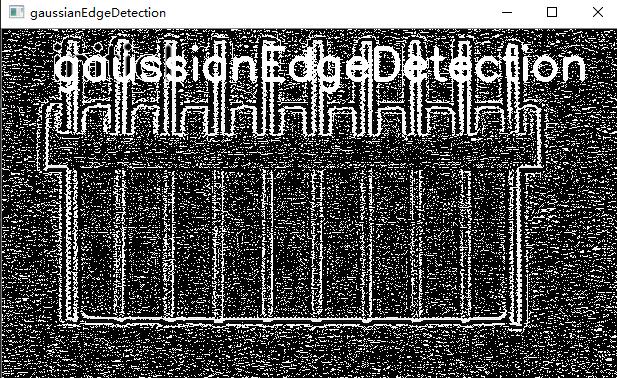
The purpose of edge detection is to identify the points with obvious brightness changes in digital images. Gauss edge detection uses Gauss filter to detect the edge.
The steps are as follows:
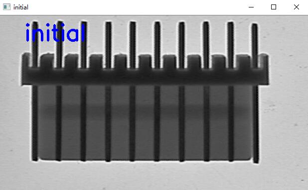
1. Read the original drawing
import cv2
import cv2 as cv

# Read the initial.bmp file in this relative path
image = cv2.imread ("initial.png")
# Add text message
cv2.putText(image,'initial',(50,50),cv2.FONT_HERSHEY_SIMPLEX,1.5,(255,0, 0),4)
# Display the image corresponding to the image in the image window
cv2.imshow('initial',image)
cv2.waitKey(0)
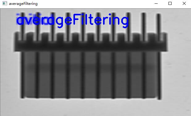
2. Mean filtering
# Mean filtering
image2 = cv2.blur(image,(10,5))
cv2.putText(image2,'averageFiltering',(50,50),cv2.FONT_HERSHEY_SIMPLEX,1.5,(255,0, 0),4)
cv2.imshow('averageFiltering',image2)
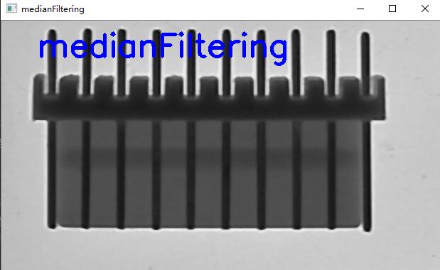
3. Median filtering
image3 = cv2.medianBlur(image, 5)
cv2.putText(image3,'medianFiltering',(50,50),cv2.FONT_HERSHEY_SIMPLEX,1.5,(255,0, 0),4)
cv2.imshow('medianFiltering',image3)
4. Gaussian filtering
After
# Gauss filtering
image4 = cv2.GaussianBlur(image,(5,5),0)
cv2.putText(image4,'gaussianFilter',(50,50),cv2.FONT_HERSHEY_SIMPLEX,1.5,(255,0, 0),4)
cv2.imshow('gaussianFilter',image4)
5. Gaussian edge detection
finally, Gaussian edge detection is carried out, and the code is as follows:
# Gaussian edge detection
gau_matrix = np.asarray([[-2/28,-5/28,-2/28],[-5/28,28/28,-5/28],[-2/28,-5/28,-2/28]])
img = np.zeros(image.shape)
hight,width = image.shape
for i in range(1,hight-1):
	for j in range(1,width-1):
		img[i-1,j-1] = np.sum(image[i-1:i+2,j-1:j+2]*gau_matrix)
image5 = img.astype(np.uint8)
cv2.putText(image5,'gaussianEdgeDetection',(50,50),cv2.FONT_HERSHEY_SIMPLEX,1.5,(255,0, 0),4)
cv2.imshow('gaussianEdgeDetection',image5)
3: Edge detection operator
Edge detection is a basic problem in image processing and computer vision. The purpose of edge detection is to identify the points with obvious brightness changes in digital images. It includes discontinuity in depth, discontinuity in surface direction, change in material properties, change in scene lighting, etc. It is a field of feature extraction in computer vision.
. The second derivative can also explain the type of gray mutation. In some cases, for example, for an image with uniform gray level change, only the first derivative may not find the boundary, and the second derivative can provide very useful information. The second derivative is also sensitive to noise. The solution is to smooth the image, eliminate some noise, and then carry out edge detection. However, the algorithm using the second derivative information is based on zero crossing detection, so the number of edge points obtained is relatively small, which is conducive to subsequent processing and recognition.
Computer vision is the process of imitating human vision. Therefore, when detecting the edge of an object, the contour points are roughly detected first, and then the original detected contour points are connected through the link rules. At the same time, the missing boundary points are detected and connected, and the false boundary points are removed. The edge of image is an important feature of image, which is the basis of computer vision and pattern recognition, so edge detection is an important part of image processing.
there are several edge detection methods in opencv, the first-order ones are Roberts Cross operator, Prewitt operator, Sobel operator, Canny operator, Krisch operator, compass operator, and the.
The steps are as follows:
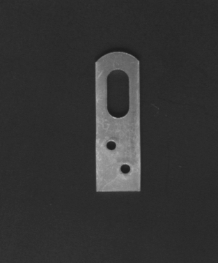
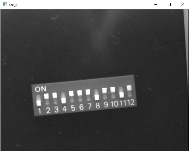
1. Display the original drawing
first show the original image with the following code:
# Read the dip switch 02.bmp file under this relative path
src_s = cv2.imread ("dip_switch_02.bmp",0)
cv2.imshow('src_s',src_s)
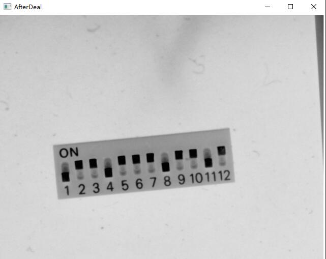
2. Reverse the image
Q Q A fter that, the image will be reversed. The code is as follows:
src = cv.imread("dip_switch_02.bmp")
height, width, channels = src.shape
for row in range(height):
    for list in range(width):
        for c in range(channels):
            pv = src[row, list, c]
            src[row, list, c] = 255 - pv
cv.imshow("AfterDeal", src)
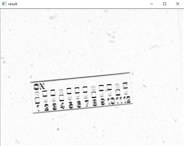
3. Image edge detection with sobel method
Sobel operator is a discrete differential operator for edge detection, which combines Gaussian smoothing and differential derivation. The operator is used to calculate the approximate value of the brightness of the image. According to the intensity of light and shade beside the edge of the image, the specific points in the area exceeding a certain number are recorded as the edge. Sobel operator adds the concept of weight on the basis of Prewitt operator, and considers that the distance between adjacent points has different influence on the current pixel. The closer the pixel is, the greater the influence on the current pixel is, so as to realize image sharpening and highlight the edge contour.
Sobel operator is more accurate in edge location, which is often used in the image with more noise and gray gradient
Sobel operator consists of two sets of 3 x 3 matrices, which are transverse and longitudinal templates. By convoluting them with the image plane, we can get the approximate luminance difference values of transverse and longitudinal respectively.
code is as follows:
# Edge detection with sobel method
x = cv2.Sobel(src,cv2.CV_16S,1,0)
y = cv2.Sobel(src,cv2.CV_16S,0,1)
absX = cv2.convertScaleAbs(x)   # Turn back to uint8
# cv2.imshow("absX", absX)

# Reverse after screenshot
def inverse_color(image):
	height, width, channels = image.shape
	for row in range(height):
			for list in range(width):
				for c in range(channels):
					pv = image[row, list, c]
					image[row, list, c] = 255 - pv

	cv.imshow("result", image)
one = cv.imread("2.jpg")
inverse_color(one)
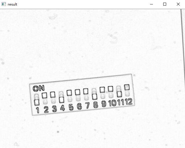
4. Image edge detection with robert method
The Roberts operator, also known as the cross differential operator, is a gradient algorithm based on the cross difference, which detects the edge line by the local difference calculation. It is often used to process low noise images with steep edges. When the edge of the image is close to the positive 45 degree or negative 45 degree, the effect of the algorithm is better. Its disadvantage is that the edge location is not very accurate, and the extracted edge line is relatively thick.
# Edge detection with robert method
dst = cv2.addWeighted(absX,0.5,absY,0.5,0)
# cv2.imshow("dst", dst)
# Reverse after screenshot
def inverse_color(image):
	height, width, channels = image.shape
	for row in range(height):
			for list in range(width):
				for c in range(channels):
					pv = image[row, list, c]
					image[row, list, c] = 255 - pv
cv.imshow("result", image)
three = cv.imread ("3.jpg")
inverse_color(three)
Four: projection
Projection is to project a scene onto the image plane of the camera. The types are perspective projection, affine projection, weak perspective projection and quasi perspective projection.
In opencv, projection is mainly divided into horizontal projection and vertical projection. Horizontal projection is the projection of two-dimensional image on the y-axis; vertical projection is the projection of two-dimensional image on the x-axis.
. The libraries used are cv2 and matplotlib.
The steps are as follows:
1. Display the original drawing
import cv2
import numpy as np
from matplotlib import pyplot as plt

img=cv2.imread('123.jpg')

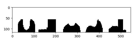
2. Vertical projection
img=cv2.imread('123.jpg') #Read the picture and replace it with an operational array
GrayImage=cv2.cvtColor(img,cv2.COLOR_BGR2GRAY) #Convert BGR image to grayscale image
ret,thresh1=cv2.threshold(GrayImage,130,255,cv2.THRESH_BINARY)#Change points between image binarization (130255) to 255 (background)
(h,w)=thresh1.shape #Return height and width
a = [0 for z in range(0, w)]
#Record the peaks of each column
for j in range(0,w): #Traversing a column
	for i in range(0,h): #Traverse a row
		if thresh1[i,j]==0: #If you change the point to black
			a[j]+=1 #Counter of this column plus one count
			thresh1[i,j]=255 #Turn it white after recording

for j in range(0,w): #Traverse each column
	for i in range((h-a[j]),h): #Start from the top point of the column that should be blackened to the bottom
		thresh1[i,j]=0 #Blackening
plt.imshow(thresh1,cmap=plt.gray())
plt.show()
cv2.imshow('one',thresh1)
cv2.waitKey(0)
3. Horizontal projection
for j in range(0,h):
	for i in range(0,w):
		if thresh1[j,i]==0:
			a[j]+=1
			thresh1[j,i]=255

for j in range(0,h):
	for i in range(0,a[j]):
		thresh1[j,i]=0

plt.imshow(thresh1,cmap=plt.gray())
plt.show()
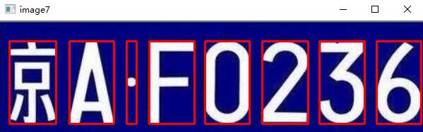
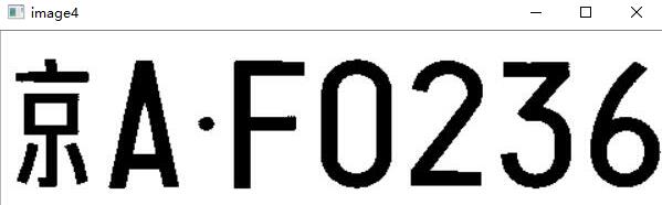
5: Character segmentation of license plate
Vehicle License Plate Recognition (VLPR) is an application of computer video image recognition technology in Vehicle License Plate Recognition.
.
. What's going on here is to identify and enclose it directly with a box. The necessary steps are first to transform the color license plate image into gray-scale image, then reverse color, threshold segmentation, and then use the horizontal and vertical projection to intercept the length and width of the required small box in order to identify. The technology used is the cv2 Library in python+opencv and the numpy library for data analysis.
The steps are as follows:
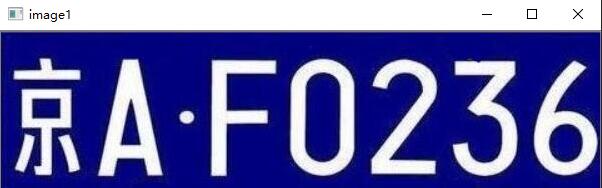
1. Read the original drawing
import cv2
import cv2 as cv
import numpy as np

image1 = cv.imread('123456.jpg',1)
cv.imshow('image1', image1)
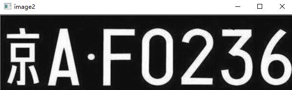
2. Gray conversion
.
image2 = cv.imread('123456.jpg',0)
cv.imshow('image2', image2)
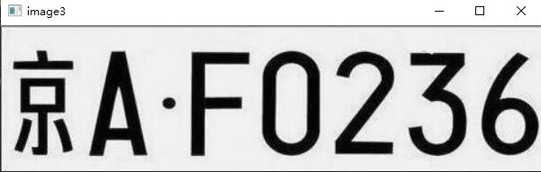
3. anti color
.
height, width, deep = image1.shape
dst = np.zeros((height,width,1), np.uint8)
for i in range(0, height):
    for j in range(0, width):
        grayPixel = image2[i, j]
        dst[i, j] = 255-grayPixel
cv2.imshow('image3', dst)
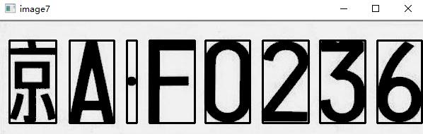
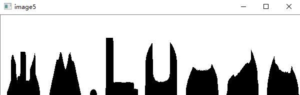
4. Threshold segmentation
.
ret, thresh = cv2.threshold(dst, 100, 255, cv2.THRESH_TOZERO)
cv2.imshow('image4', thresh)
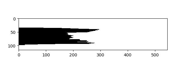
5. projection
After .
# Horizontal projection
def hProject(binary):
    h, w = binary.shape
    # Horizontal projection
    hprojection = np.zeros(binary.shape, dtype=np.uint8)
    # Create an array with h length of 0
    h_h = [0]*h
    for j in range(h):
        for i in range(w):
            if binary[j,i] == 0:
                h_h[j] += 1
    # Draw a projection
    for j in range(h):
        for i in range(h_h[j]):
            hprojection[j,i] = 255
    return h_h

# Vertical back projection
def vProject(binary):
    h, w = binary.shape
    # Vertical projection
    vprojection = np.zeros(binary.shape, dtype=np.uint8)
    # Create an array with w length of 0
    w_w = [0]*w
    for i in range(w):
        for j in range(h):
            if binary[j, i ] == 0:
                w_w[i] += 1
    for i in range(w):
        for j in range(w_w[i]):
            vprojection[j,i] = 255
    return w_w

6. Character recognition matching and segmentation
.
th = thresh
h,w = th.shape
h_h = hProject(th)
start = 0
h_start, h_end = [], []
position = []
# Vertical segmentation based on horizontal projection
for i in range(len(h_h)):
    if h_h[i] > 0 and start == 0:
        h_start.append(i)
        start = 1
    if h_h[i] ==0 and start == 1:
        h_end.append(i)
        start = 0
for i in range(len(h_start)):
    cropImg = th[h_start[i]:h_end[i], 0:w]
    if i ==0:
        pass
    w_w = vProject(cropImg)
    wstart , wend, w_start, w_end = 0, 0, 0, 0
    for j in range(len(w_w)):
        if w_w[j] > 0 and wstart == 0:
            w_start = j
            wstart = 1
            wend = 0
        if w_w[j] ==0 and wstart == 1:
            w_end = j
            wstart = 0
            wend = 1
        # Save coordinates when start and end points are confirmed
        if wend == 1:
            position.append([w_start, h_start[i], w_end, h_end[i]])
            wend = 0
# Determine division position
for p in position:
    cv2.rectangle(thresh, (p[0], p[1]), (p[2], p[3]), (0, 0, 255), 2)
cv2.imshow('image7', thresh)
cv.waitKey(0)