Naive Bayes

The joint probability P(A,B) = P(B|A)*P(A) = P(A|B)*P(B) combines the two equations on the right to get the following formula:

P (a| b) indicates the probability of a in the case of B. P(A|B) = [P(B|A)*P(A)] / P(B)

Let's have A visual understanding of this formula. As shown in the figure below, the probability of problem A changes after we know the information of B (the picture comes from The easy to understand Bayes' Theorem of Xiaobai)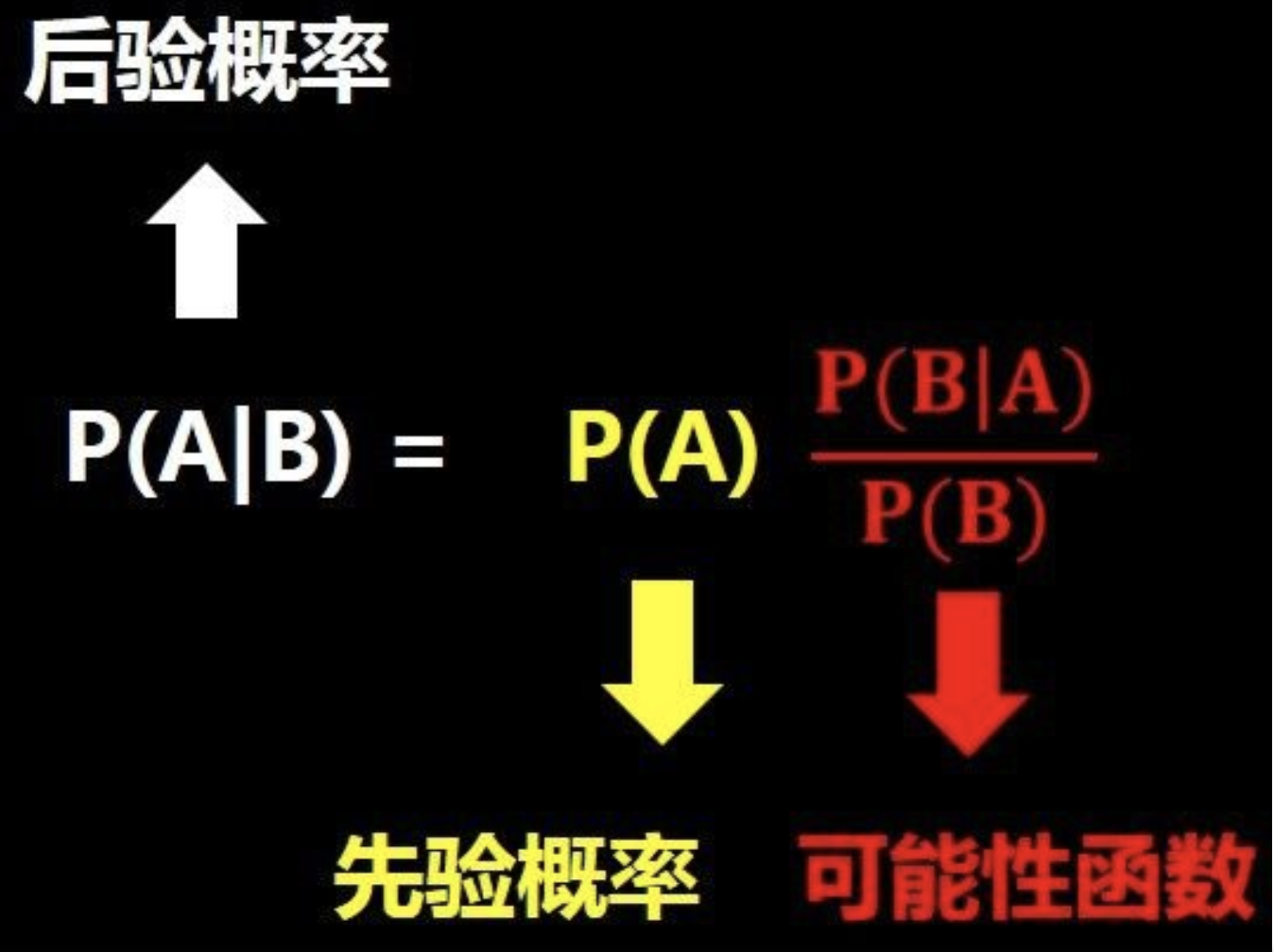

1. Posterior probability derivation

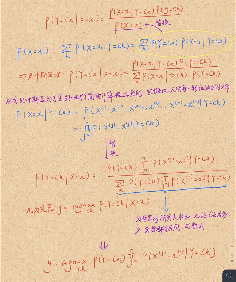
Naive Bayes condition: each characteristic term of vector X is independent and identically distributed. This condition is too broad, but in order to make calculation simple, we try to use it. After using it, we find that the effect is good, so use it

2. Maximum likelihood estimation to get y value of classifier

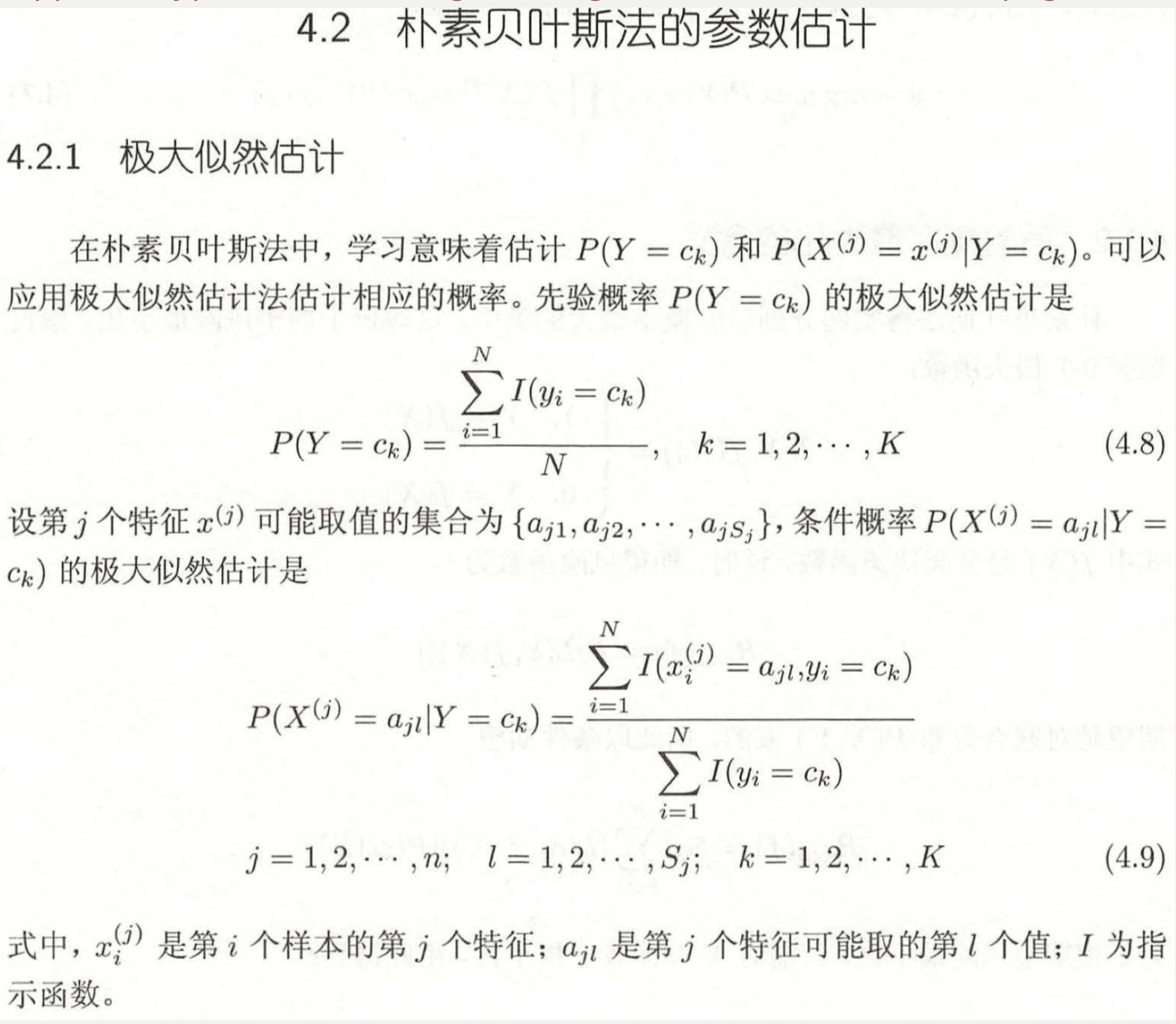
Do you remember the formula of finding the maximum probability under different categories (classifier y)? There's a lot of riders in there remember?

Here is a question. What if one of the multiple probabilities is 0? So the whole formula is zero directly. That's not right. So we have to find a way to ensure that every item in the multiplication is not 0, even if it was originally 0. (if it was originally 0, it means that it has the smallest probability among all the multiplication items, so long as it still has the smallest value after the conversion, it has no impact on the size of the result.) here we use Bayesian estimation.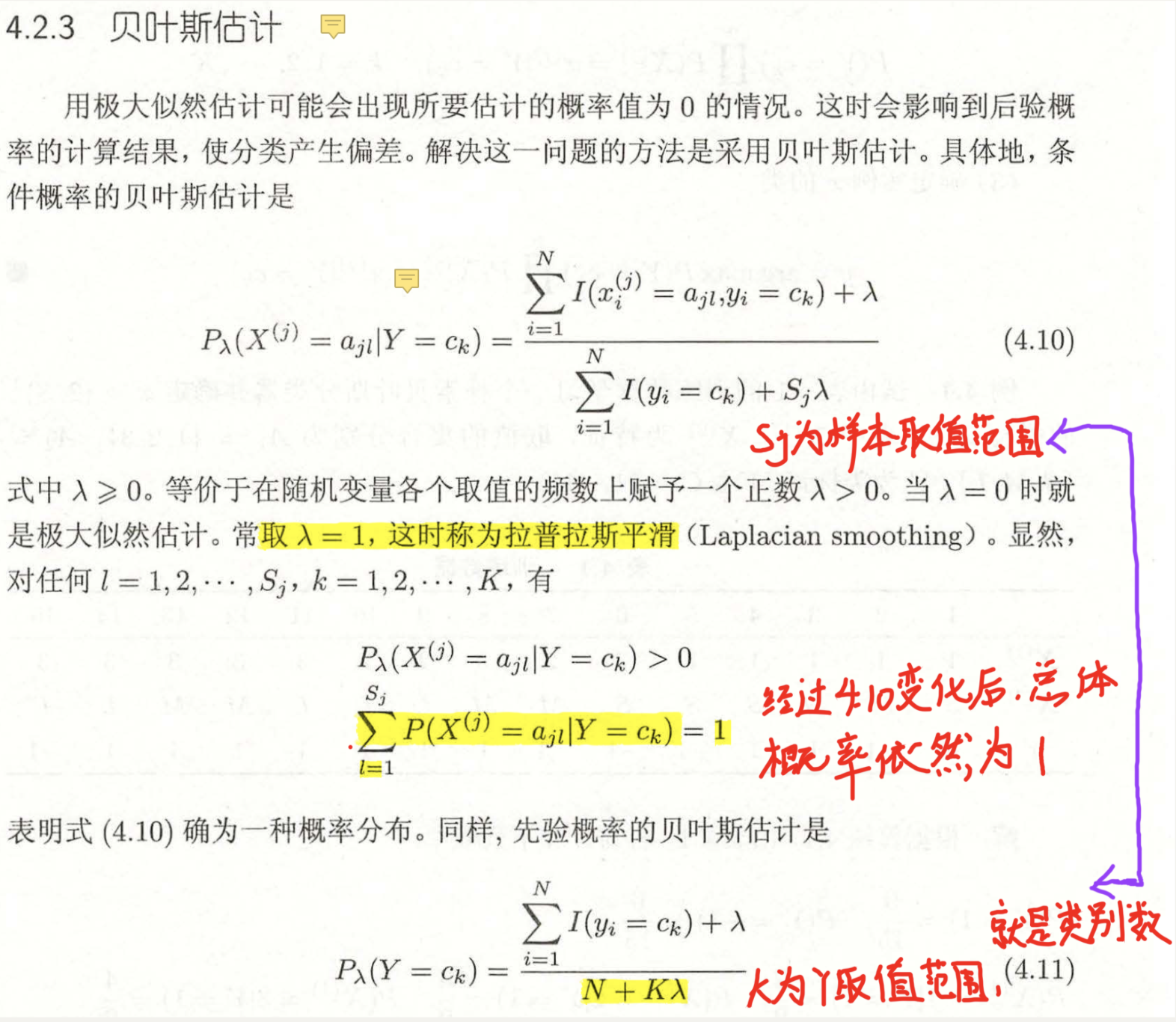

The purpose of this transformation is that each probability is not zero, so it has no effect on the formula of y-multiplication. However, in order to keep the sum of probability values still 1, it has evolved into the above formula

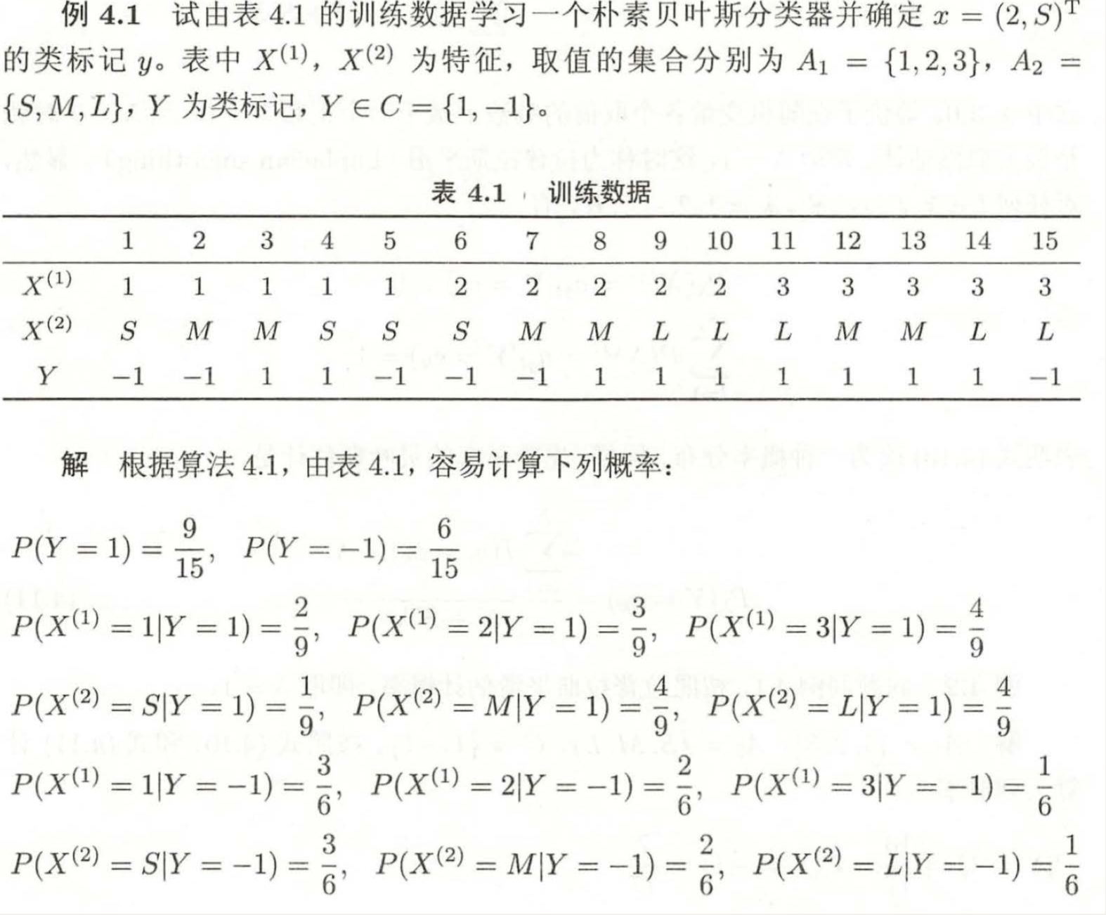
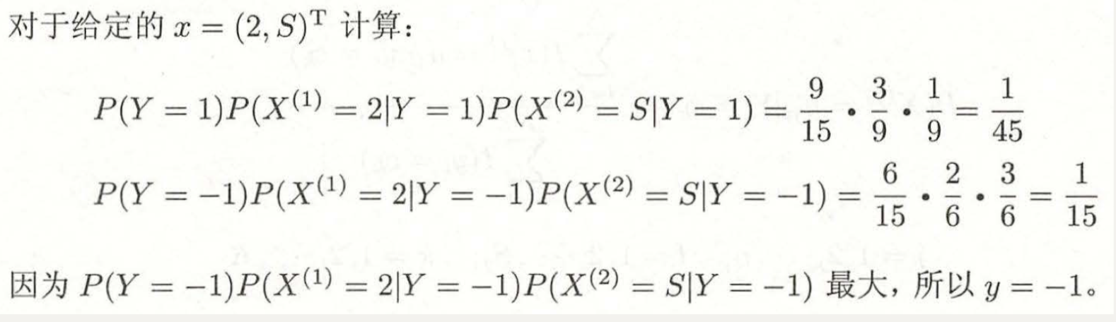
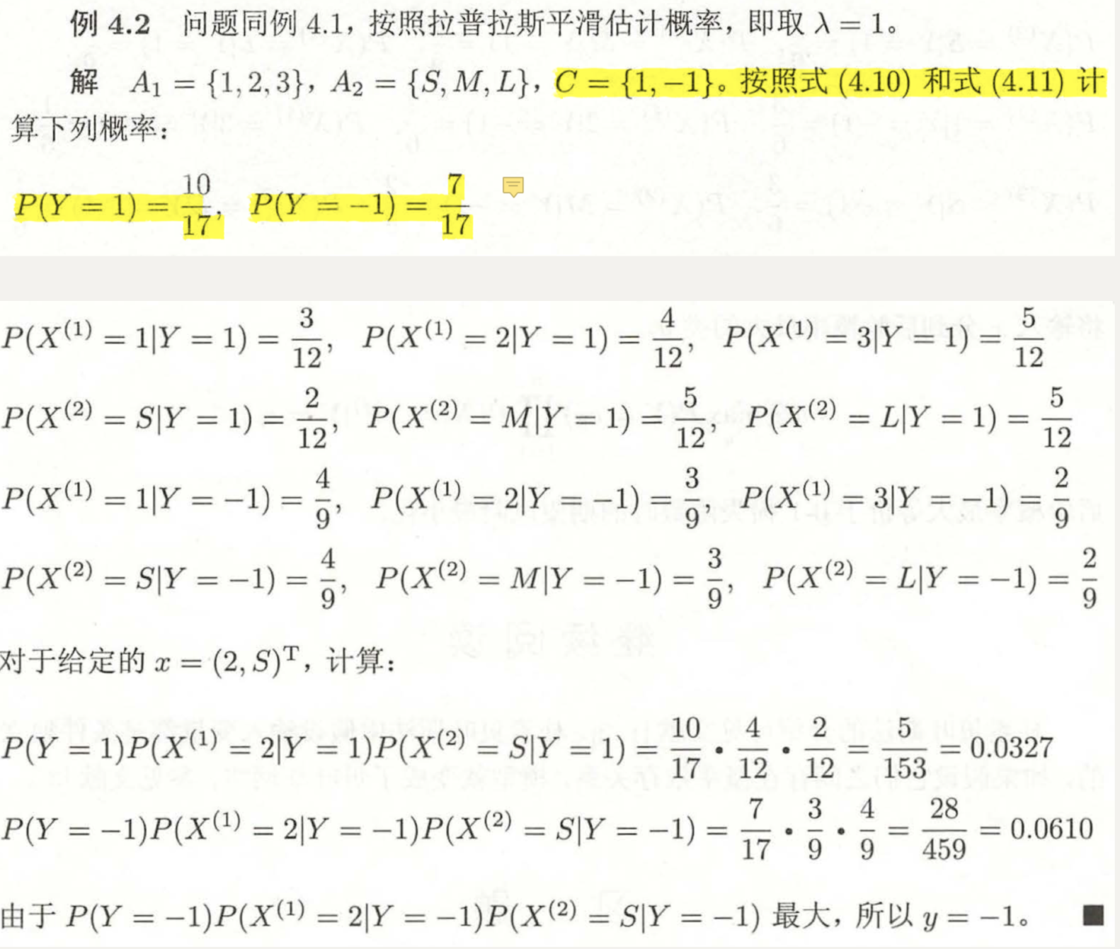
3. Example understanding

3.1 naive Bayes

3.2 Bayesian estimation

4. supplement

In practice, it is not only necessary to use Bayesian estimation (the probability of guarantee is not 0), but also to take logarithm (to ensure that the result of multiplication does not overflow).

Why?

Since the multiplication terms are all between 0-1, many (characteristic number) numbers between 0-1 are multiplied, and the final number must be very small, which may be infinitely close to 0. For a program, too close to zero may cause a lower overflow, which means that the precision is not enough. So we will take the logarithm of the whole multiplication term, so that even if the final result of all multiplication is infinitely close to 0, the number will become very large (although it is negative) after taking the log, and the computer can express it.

Will the result change after log ging?

The answer is No. Log is an increasing function in the domain of definition, and X in log(x) is also an increasing function. In the case of the same monotonicity, the result of multiplication is large, and the log is also large, which does not affect the comparison of different multiplication results

5. Code reproduction (jupyter)

#Download MINST handwriting dataset and load
import tensorflow as tf
mnist = tf.keras.datasets.mnist
(X_train, y_train), (X_test, y_test) = mnist.load_data()

#X_train.shape is (60000, 28, 28)
#y_train.shape is (60000,)
#Let's expand the data
X_train = X_train.reshape(-1 , 28*28)
y_train = y_train.reshape(-1 , 1)
X_test = X_test.reshape(-1 , 28*28)
y_test = y_test.reshape(-1 , 1)

#For simplicity, let's binarize the handwritten data picture
X_train[X_train <  128] = 0
X_train[X_train >= 128] = 1
X_test[X_test <  128] = 0
X_test[X_test >= 128] = 1

import numpy as np
#According to the formula, the prior probability p_yis calculated, and the Laplace smoothing λ = 1 is used, and the log is taken for the multiplication formula
P_y = np.zeros((10 , 1))
classes = 10
for i in range(classes):
    P_y[i] = ((np.sum(y_train == i))+1)/(len(y_train)+classes)
P_y = np.log(P_y)
print(P_y)

#Calculate conditional probability Px_y
#This module can calculate the number of each eigenvalue
Px_y = np.zeros((classes , X_train.shape[1] , 2))
for i in range(X_train.shape[0]):
    k = y_train[i]
    x = X_train[i]
    for feature in range(X_train.shape[1]):
        Px_y[k,feature,x[f]] += 1       

#Start to calculate the conditional probability Px_y
#
for index in range(classes):
    for f in range(X_train.shape[1]):
        Px_y[index , f , 0] = (Px_y[index , f , 0] + 1) / (np.sum(y_train == index) + 2)
        Px_y[index , f , 1] = (Px_y[index , f , 1] + 1) / (np.sum(y_train == index) + 2)
#In order to change the multiplication into the addition, we take a log logarithm for Px_y
Px_y = np.log(Px_y)
#Take one out and have a look
print(Px_y[0])

#The final result of our prediction is put in predict
#The results of each data in 10 classifiers are put in res, and one argmax is taken to get a prediction value
predict = np.zeros((y_test.shape[0],1))
for data in range(y_test.shape[0]):
    res = np.zeros((classes , 1))
    for i in range(classes):
        res[i] = P_y[i]
        for f in range(X_train.shape[1]):
            res[i] += Px_y[i,f,X_test[data,f]]
    predict[data] = np.argmax(res)
predict = predict.astype(int)
#Take two and compare them
print(predict[:5])
print(y_test[:5])

#Predict the accuracy
precision = np.sum(predict == y_test) / y_test.shape[0]
print(precision)

Please like it if you think it's useful

Reference article:
Li Hang's statistical learning method (Second Edition)
Statistical learning method analysis and implementation of naive Bayes principle