premise
Language: python
Framework: tensorflow
The introduction of in-depth learning is handwritten digit recognition, which is the same as the first helloworld of our language
You, the most basic and the least white, should start with the Keras framework. The background of the Keras framework is tensorflow
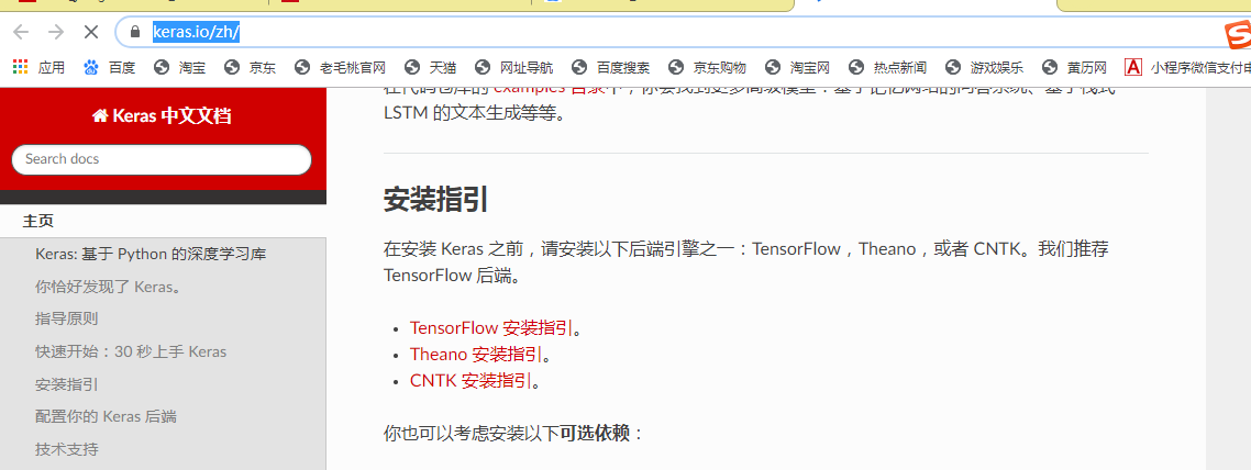
For Python installation, Tensorflow installation and Keras framework installation, see the official website here https://keras.io/zh/
The whole idea of handwritten digit recognition is as follows
In the data set, the training set (such as the picture with the number 5), the corresponding label of the training set (such as 5), the test set, and the corresponding label of the test set;
The training set is used to train the model, and the test set is used to evaluate the performance of the model. The model loads the pictures of the test set, predicts the numbers on the pictures, and then validates the labels corresponding to the test set. If the accuracy is high, the performance of the model is excellent.
Note: the machine does not know or understand pictures. It imitates the learning process of human brain nerves. After the hidden layer, it outputs a predicted value through the output layer to check the pictures corresponding to the training set, constantly adjust the error, improve the recognition rate, and achieve the effect of intelligent recognition!
Of course, many terms such as loss function, optimization function, random gradient descent, full connection layer, convolution layer, pooling layer and so on. If you understand all of them before you start, I think you don't want to start. You are tired. So let's first learn about deep learning through a simple example, and then learn various algorithms.
First, we import the mnist data set we need from the data set of keras framework;
The pictures in the mnist data set are handwritten pictures of all kinds of people collected by American researchers, with the recognition rate of 99%. It is the same major as the textbook;
If we do our own voiceprint recognition, the best data set can be downloaded from the Internet;
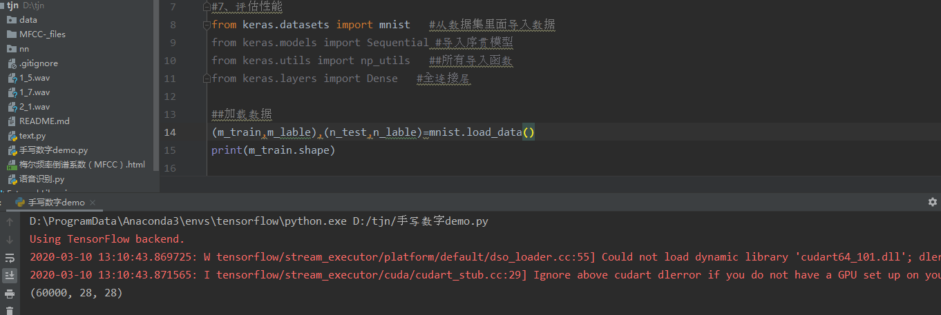
Step 1: load the dataset
M'train is a training set picture, 60000 in total, each picture is 28 * 28 in width and height, which is a gray picture;
M? Lable is the label corresponding to the training set picture (the number is between 0-9)
n_test is the test set picture, a total of 10000 pictures, each of which is 28 * 28 in width and height, and is a gray-white picture
N? Label is the label corresponding to the test set picture (the number is between 0-9)
mnist.load_data() is the loading data set. If there is no program, it will be automatically downloaded from the Internet. The name is mnist.npz
If so, the data will be loaded automatically
m_train.shape is the shape of training set. The first 60000 is the number of pictures, the second is width, and the third is height;
Step 2: preprocessing training set and test set
2.1. Our pictures are (28, 28), but in-depth learning, we mainly use the whole picture, which should be 28 * 28 = 784
2.2. The label is 0-9, 10 types. These 10 types have no size discrimination before. For the sake of this, they all become one hot form
One hot is
If it's three categories, it's 100 010 001
If it's class 4, it's 1000 0100 0010 0001
##Processing pictures
m_train=m_train.reshape(m_train.shape[0],-1)
n_test=n_test.reshape(n_test.shape[0],-1)
##One hot coding
m_lable=np_utils.to_categorical(m_lable,num_classes=10)
n_lable=np_utils.to_categorical(n_lable,num_classes=10)
Step 3: create a model and add a hidden layer
units=512 refers to 512 neurons. When there is only the first layer, the input input dim=784 needs to be specified;
##Create a sequential model
model=Sequential()
# ##Input layer does not need to be added
model.add(Dense(units=512,input_dim=784,activation='relu'))
model.add(Dense(units=512,activation='relu'))
# ##Output layer
model.add(Dense(units=10,activation='softmax'))
The fourth step, loss algorithm and optimization algorithm
model.compile(loss='categorical_crossentropy',optimizer='Adam',metrics=['accuracy'])
model.fit(m_train,m_lable,batch_size=50,epochs=3)
Step 5: use test set to evaluate the model
##Evaluate trained models
loss,mm=model.evaluate(n_test,n_lable)
print(loss,mm)
Now attach the complete code
from keras.datasets import mnist   #Import data from dataset
from keras.models import Sequential #Import sequential model
from keras.utils import np_utils   ##All import functions
from keras.layers import Dense   #Fully connected layer
##Loading data
(m_train,m_lable),(n_test,n_lable)=mnist.load_data()
print(m_train.shape)
##Processing pictures
m_train=m_train.reshape(m_train.shape[0],-1)
n_test=n_test.reshape(n_test.shape[0],-1)
##One hot coding
m_lable=np_utils.to_categorical(m_lable,num_classes=10)
n_lable=np_utils.to_categorical(n_lable,num_classes=10)
##Create a sequential model
model=Sequential()
# ##Input layer does not need to be added
model.add(Dense(units=512,input_dim=784,activation='relu'))
model.add(Dense(units=512,activation='relu'))
# ##Output layer
model.add(Dense(units=10,activation='softmax'))
# ##Optimize and reduce losses
model.compile(loss='categorical_crossentropy',optimizer='Adam',metrics=['accuracy'])
model.fit(m_train,m_lable,batch_size=50,epochs=3)
##Evaluate trained models
loss,mm=model.evaluate(n_test,n_lable)
print(loss,mm)
##Training model for given input
model.save('tjn.h5')
Now, we can run the program, train and evaluate the model
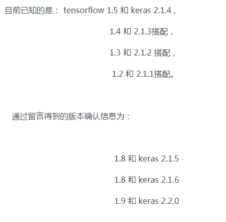
Module 'tensorflow' has no attribute 'get default' graph 'will be reported as soon as the program is running
The reason is that the version of tensorflow is incompatible with the version of keras. At this time, we need to reduce or increase the version of keras
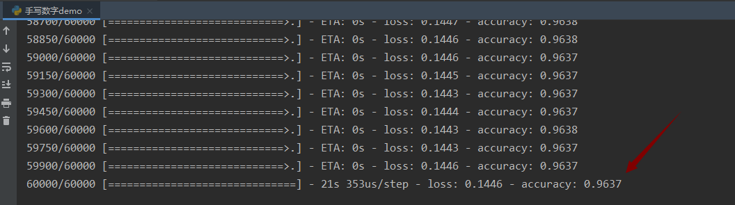
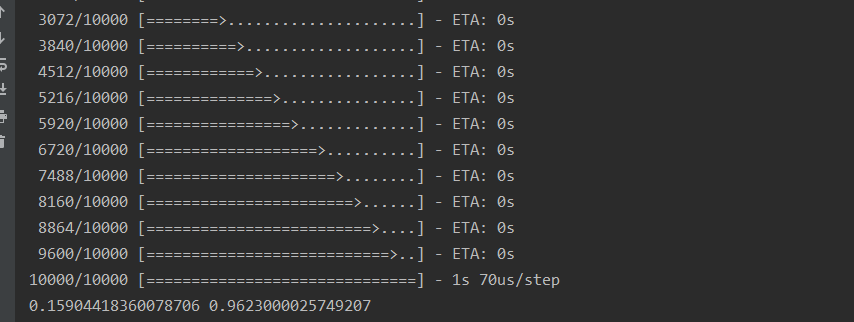
The operation results are as follows
The accuracy of the training model is 96.37%
The accuracy is 96.23%
Is the head still dizzy?
What's the loss function, the optimization function, the neuron? What's the matter?
If you know it now, you don't have to learn
After you knock it out first, and then run it, we'll discuss the random gradient algorithm and back propagation in the next article!

