Home Credit Default Risk
conclusion
The data is provided by Home Credit (Chinese Name: Home Credit), which is dedicated to providing credit to people without bank accounts. The task requires forecasting whether the customer will repay the loan or encounter difficulties. AUC (ROC) is used as the evaluation standard of the model.
This blog only analyzes the application train / application test data, and uses Logistic Regression for classification and prediction. The results of public board 0.749 and private board 0.748 can be obtained by grid search. The Baseline is 0.68810, with a best score of 0.79857. The rest is in advanced level.
background knowledge
Home Credit is one of the leading consumer finance providers in central and Eastern Europe and Asia. It serves consumers in central and Eastern Europe (CEE), Russia, CIS and Asia.
Querying users' historical credit records in credit agencies can be used as a reference for risk assessment, but the credit data is often incomplete, because these people themselves have few bank records. The data set bureau.csv and bureau balance.csv correspond to this part of data.
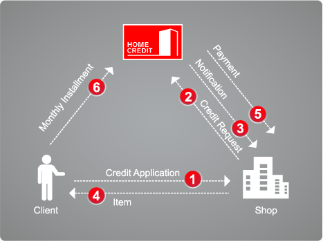
There are three types of Home Credit products: credit card, POS (consumer loan) and cash loan. Credit cards are popular in Europe and the United States, but not in those countries. Therefore, the credit card data in the data set is less. POS can only buy things, cash loans can get cash. All three types of products have application and repayment records. In the data set, previous_application.csv, POS_CASH_BALANCE.csv, credit_card_balance.csv, installations_payment.csv correspond to this part of data.
The English versions of the three types of products are: Revolving loan (credit card), consumer installation loan (point of sales loan – POS loan), installation cash loan.
data set
According to the introduction above, data set includes 8 different data files, which can be divided into three categories.
-
application_train, application_test:
The training set includes information about each loan application of Home Credit. Each loan has its own line and is identified by SK? ID? Curr. TARGET 0 of training set: the loan has been paid off, 1: the loan has not been paid off.
Through these two files, we can do basic data analysis and modeling for this task, which is also the content of this blog. -
bureau, bureau_balance:
These two documents are provided by credit agencies, the user's loan application data in other financial institutions, and the monthly repayment arrears record. A user (SK ﹣ ID ﹣ curr) can have multiple loan application data (SK ﹣ ID ﹣ Bureau). -
previous_application, POS_CASH_BALANCE,credit_card_balance,installments_payment
These four files are from Home Credit. Users may have used POS services, credit cards, and applied for loans at Home Credit. These documents are the relevant application data and repayment records. A user can have multiple historical data (SK ID prev).
The following figure shows how all the data are related, and links the three parts of data through three IDS, SK ﹣ ID ﹣ curr, SK ﹣ ID ﹣ Breau and SK ﹣ ID ﹣ prev.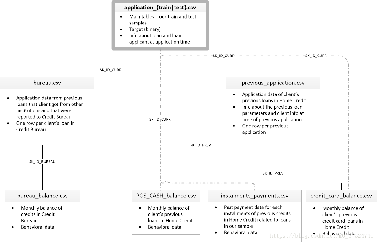
Data analysis
Balance degree
Read data from application train and application test. There are 307511 data and 122 features in the training set. Among them, the number of defaults (Target = 1) is 24825, and the number of no defaults (Target = 0) is 282686. The imbalance is not serious.
# -*- coding: utf-8 -*-

##307511, 1220, 300000 data, 280000, 21000, this imbalance is not serious
app_train = pd.read_csv('input/application_train.csv')
app_test = pd.read_csv('input/application_test.csv')
print('training data shape is', app_train.shape)
print(app_train['TARGET'].value_counts())
training data shape is (307511, 122)
0    282686
1     24825
Name: TARGET, dtype: int64
Missing data
Of the 122 features, 67 were missing, of which 49 were missing more than 47%.
## 67 features are missing and 49 data are missing more than 47%. 47 of them are related to housing features. Can we use PCA to reduce this housing feature. See what others do with it.
## ext_source and own_car_age are left. Or these 49 features can be deleted.
mv = app_train.isnull().sum().sort_values()
mv = mv[mv>0]
mv_rate = mv/len(app_train)
mv_df = pd.DataFrame({'mv':mv, 'mv_rate':mv_rate})
print('number of features with more than 47% missing', len(mv_rate[mv_rate>0.47]))
mv_rate[mv_rate> 0.47]
number of features with more than 47% missing 49

EMERGENCYSTATE_MODE             0.473983
TOTALAREA_MODE                  0.482685
YEARS_BEGINEXPLUATATION_MODE    0.487810
YEARS_BEGINEXPLUATATION_AVG     0.487810
YEARS_BEGINEXPLUATATION_MEDI    0.487810
FLOORSMAX_AVG                   0.497608
FLOORSMAX_MEDI                  0.497608
FLOORSMAX_MODE                  0.497608
HOUSETYPE_MODE                  0.501761
LIVINGAREA_AVG                  0.501933
LIVINGAREA_MODE                 0.501933
LIVINGAREA_MEDI                 0.501933
ENTRANCES_AVG                   0.503488
ENTRANCES_MODE                  0.503488
ENTRANCES_MEDI                  0.503488
APARTMENTS_MEDI                 0.507497
APARTMENTS_AVG                  0.507497
APARTMENTS_MODE                 0.507497
WALLSMATERIAL_MODE              0.508408
ELEVATORS_MEDI                  0.532960
ELEVATORS_AVG                   0.532960
ELEVATORS_MODE                  0.532960
NONLIVINGAREA_MODE              0.551792
NONLIVINGAREA_AVG               0.551792
NONLIVINGAREA_MEDI              0.551792
EXT_SOURCE_1                    0.563811
BASEMENTAREA_MODE               0.585160
BASEMENTAREA_AVG                0.585160
BASEMENTAREA_MEDI               0.585160
LANDAREA_MEDI                   0.593767
LANDAREA_AVG                    0.593767
LANDAREA_MODE                   0.593767
OWN_CAR_AGE                     0.659908
YEARS_BUILD_MODE                0.664978
YEARS_BUILD_AVG                 0.664978
YEARS_BUILD_MEDI                0.664978
FLOORSMIN_AVG                   0.678486
FLOORSMIN_MODE                  0.678486
FLOORSMIN_MEDI                  0.678486
LIVINGAPARTMENTS_AVG            0.683550
LIVINGAPARTMENTS_MODE           0.683550
LIVINGAPARTMENTS_MEDI           0.683550
FONDKAPREMONT_MODE              0.683862
NONLIVINGAPARTMENTS_AVG         0.694330
NONLIVINGAPARTMENTS_MEDI        0.694330
NONLIVINGAPARTMENTS_MODE        0.694330
COMMONAREA_MODE                 0.698723
COMMONAREA_AVG                  0.698723
COMMONAREA_MEDI                 0.698723
dtype: float64
data type
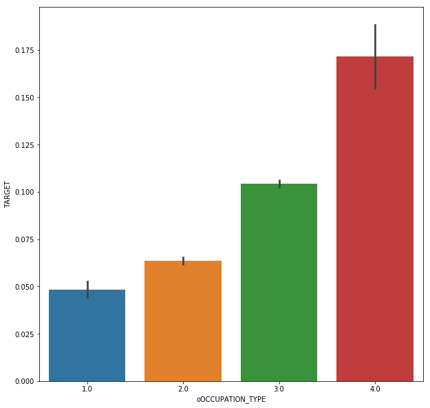
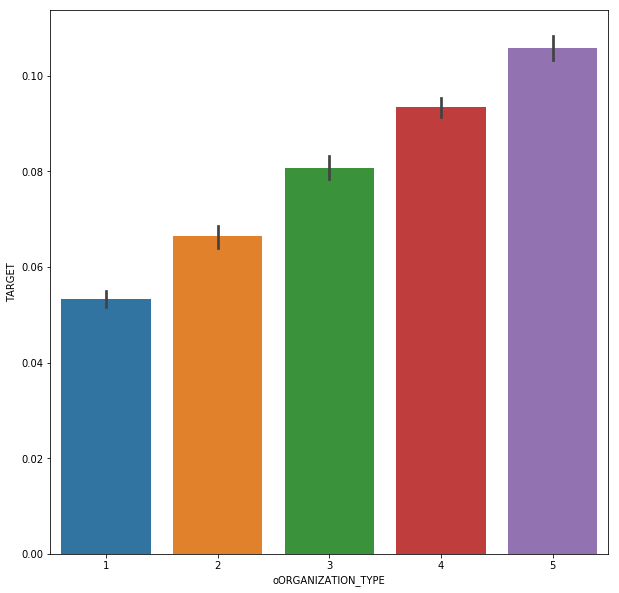
Of the 122 features, 65 are floating-point types, 41 are integer types, and 16 are non data features. The relationship between non data type feature and Target is analyzed. Occupation ﹣ type and organization ﹣ type can be manually coded, and the rest can be directly encoded by Onehot encoding.
## 65 floating-point, 41 integer, 16 non data features, except for location¢type and organization¢type, the rest should be able to be manually encoded
categorical = [col for col in app_train.columns if app_train[col].dtypes == 'object']
ct = app_train[categorical].nunique().sort_values()
for col in categorical:
    if (col!='OCCUPATION_TYPE') & (col!='ORGANIZATION_TYPE'):
        plt.figure(figsize = [10,10])
        sns.barplot(y = app_train[col], x = app_train['TARGET'])
# For the feature code with the feature number of 2, nunique is different from len(unique). The former does not calculate null, and the latter will calculate null
from sklearn.preprocessing import LabelEncoder
lb = LabelEncoder()
count = 0
for col in categorical:
    if len(app_train[col].unique()) == 2:
        count = count + 1
        lb.fit(app_train[col])
        app_train['o' + col] = lb.transform(app_train[col])
        app_test['o' + col] = lb.transform(app_test[col])
# The overdue rate of housing type mode and family status is related to the classification.
# OCCUPATION can be coded as follows
col = 'OCCUPATION_TYPE'
#occ_sort = app_train.groupby(['OCCUPATION_TYPE'])['TARGET'].agg(['mean','count']).sort_values(by = 'mean')
#order1 = list(occ_sort.index)
#plt.figure(figsize = [10,10])
#sns.barplot(y = app_train[col], x = app_train['TARGET'], order = order1)
dict1 = {'Accountants' : 1,
         'High skill tech staff':2, 'Managers':2,  'Core staff':2,
         'HR staff' : 2,'IT staff': 2, 'Private service staff': 2, 'Medicine staff': 2,
          'Secretaries': 2,'Realty agents': 2,
          'Cleaning staff': 3, 'Sales staff': 3,  'Cooking staff': 3,'Laborers': 3,
          'Security staff': 3,  'Waiters/barmen staff': 3,'Drivers': 3,
          'Low-skill Laborers': 4}
app_train['oOCCUPATION_TYPE'] = app_train['OCCUPATION_TYPE'].map(dict1)
app_test['oOCCUPATION_TYPE'] = app_test['OCCUPATION_TYPE'].map(dict1)
plt.figure(figsize = [10,10])
sns.barplot(x = app_train['oOCCUPATION_TYPE'], y = app_train['TARGET'])
##
col = 'ORGANIZATION_TYPE'
#organ_sort = app_train.groupby(['ORGANIZATION_TYPE'])['TARGET'].agg(['mean','count']).sort_values(by = 'mean')
#order1 = list(organ_sort.index)
#plt.figure(figsize = [20,20])
#sns.barplot(y = app_train[col], x = app_train['TARGET'], order = order1)

dict1 = {'Trade: type 4' :1,  'Industry: type 12' :1,  'Transport: type 1' :1,  'Trade: type 6' :1,
 'Security Ministries' :1,  'University' :1,  'Police' :1,  'Military' :1, 'Bank' :1, 'XNA' :1,

 'Culture' :2,  'Insurance' :2, 'Religion' :2,  'School' :2,  'Trade: type 5' :2, 'Hotel' :2, 'Industry: type 10' :2,
 'Medicine' :2,  'Services' :2,  'Electricity' :2,  'Industry: type 9' :2,  'Industry: type 5' :2, 'Government' :2,
 'Trade: type 2' :2, 'Kindergarten' :2, 'Emergency' :2, 'Industry: type 6' :2, 'Industry: type 2' :2, 'Telecom' :2,

 'Other' :3, 'Transport: type 2' :3, 'Legal Services' :3, 'Housing' :3, 'Industry: type 7' :3, 'Business Entity Type 1' :3,
 'Advertising' :3, 'Postal':3, 'Business Entity Type 2' :3, 'Industry: type 11' :3, 'Trade: type 1' :3, 'Mobile' :3,

 'Transport: type 4' :4, 'Business Entity Type 3' :4, 'Trade: type 7' :4, 'Security' :4, 'Industry: type 4' :4,

 'Self-employed' :5, 'Trade: type 3' :5, 'Agriculture' :5, 'Realtor' :5, 'Industry: type 3' :5, 'Industry: type 1' :5,
 'Cleaning' :5, 'Construction' :5, 'Restaurant' :5, 'Industry: type 8' :5, 'Industry: type 13' :5, 'Transport: type 3' :5}
app_train['oORGANIZATION_TYPE'] = app_train['ORGANIZATION_TYPE'].map(dict1)
app_test['oORGANIZATION_TYPE'] = app_test['ORGANIZATION_TYPE'].map(dict1)
plt.figure(figsize = [10,10])
sns.barplot(x = app_train['oORGANIZATION_TYPE'], y = app_train['TARGET'])

## The rest of them are ohe(307511, 127),(48744, 126) drop, and the feature s are 122121
discard_features = ['ORGANIZATION_TYPE', 'OCCUPATION_TYPE','FLAG_OWN_CAR','FLAG_OWN_REALTY','NAME_CONTRACT_TYPE']
app_train.drop(discard_features,axis = 1, inplace = True)
app_test.drop(discard_features,axis = 1, inplace = True)
# Then use get Dummies (307511, 169) (48744, 165)
app_train = pd.get_dummies(app_train)
app_test = pd.get_dummies(app_test)
print('Training Features shape: ', app_train.shape)
print('Testing Features shape: ', app_test.shape)
# Some features are not included in the test and need to be aligned (307511, 166) (48744, 165)
train_labels = app_train['TARGET']
app_train, app_test = app_train.align(app_test, join = 'inner', axis = 1)
app_train['TARGET'] = train_labels

print('Training Features shape: ', app_train.shape)
print('Testing Features shape: ', app_test.shape)
Training Features shape:  (307511, 169)
Testing Features shape:  (48744, 165)
Training Features shape:  (307511, 166)
Testing Features shape:  (48744, 165)
Outliers
Abnormal data is found in the feature days employee, which has a strong correlation with Target and needs special processing. In addition, add a feature, days? Employee? Anom, to indicate whether the feature is abnormal. This processing should be more effective for linear methods, and tree based methods should be able to identify automatically.
## Continue to EDA, and find the problem data in the days employee. This processing should be effective for the linear method, and the boost method should be able to identify automatically.
app_train['DAYS_EMPLOYED'].plot.hist(title = 'DAYS_EMPLOYMENT HISTOGRAM')
app_test['DAYS_EMPLOYED'].plot.hist(title = 'DAYS_EMPLOYMENT HISTOGRAM')
app_train['DAYS_EMPLOYED_ANOM'] = app_train['DAYS_EMPLOYED'] == 365243
app_train['DAYS_EMPLOYED'].replace({365243: np.nan}, inplace = True)
app_test['DAYS_EMPLOYED_ANOM'] = app_test["DAYS_EMPLOYED"] == 365243
app_test["DAYS_EMPLOYED"].replace({365243: np.nan}, inplace = True)

app_train['DAYS_EMPLOYED'].plot.hist(title = 'Days Employment Histogram');
plt.xlabel('Days Employment')

## Extract correlation
correlations = app_train.corr()['TARGET'].sort_values()
print('Most Positive Correlations:\n', correlations.tail(15))
print('\nMost Negative Correlations:\n', correlations.head(15))
Most Positive Correlations:
 REG_CITY_NOT_LIVE_CITY                               0.044395
FLAG_EMP_PHONE                                       0.045982
NAME_EDUCATION_TYPE_Secondary / secondary special    0.049824
REG_CITY_NOT_WORK_CITY                               0.050994
DAYS_ID_PUBLISH                                      0.051457
CODE_GENDER_M                                        0.054713
DAYS_LAST_PHONE_CHANGE                               0.055218
NAME_INCOME_TYPE_Working                             0.057481
REGION_RATING_CLIENT                                 0.058899
REGION_RATING_CLIENT_W_CITY                          0.060893
oORGANIZATION_TYPE                                   0.070121
DAYS_EMPLOYED                                        0.074958
oOCCUPATION_TYPE                                     0.077514
DAYS_BIRTH                                           0.078239
TARGET                                               1.000000
Name: TARGET, dtype: float64

Most Negative Correlations:
 EXT_SOURCE_3                           -0.178919
EXT_SOURCE_2                           -0.160472
EXT_SOURCE_1                           -0.155317
NAME_EDUCATION_TYPE_Higher education   -0.056593
CODE_GENDER_F                          -0.054704
NAME_INCOME_TYPE_Pensioner             -0.046209
DAYS_EMPLOYED_ANOM                     -0.045987
FLOORSMAX_AVG                          -0.044003
FLOORSMAX_MEDI                         -0.043768
FLOORSMAX_MODE                         -0.043226
EMERGENCYSTATE_MODE_No                 -0.042201
HOUSETYPE_MODE_block of flats          -0.040594
AMT_GOODS_PRICE                        -0.039645
REGION_POPULATION_RELATIVE             -0.037227
ELEVATORS_AVG                          -0.034199
Name: TARGET, dtype: float64
Fill in missing values
## Feature Engineering
## Fill in missing values
from sklearn.preprocessing import Imputer, MinMaxScaler
imputer = Imputer(strategy = 'median')
scaler = MinMaxScaler(feature_range = [0,1])
train = app_train.drop(columns = ['TARGET'])

imputer.fit(train)
train = imputer.transform(train)
test = imputer.transform(app_test)
scaler.fit(train)
train = scaler.transform(train)
test = scaler.transform(test)
print('Training data shape: ', train.shape)
print('Testing data shape: ', test.shape)
D:\Anaconda3\lib\site-packages\sklearn\utils\deprecation.py:66: DeprecationWarning: Class Imputer is deprecated; Imputer was deprecated in version 0.20 and will be removed in 0.22. Import impute.SimpleImputer from sklearn instead.
  warnings.warn(msg, category=DeprecationWarning)


Training data shape:  (307511, 166)
Testing data shape:  (48744, 166)
modeling
Logistic Regression
The results show that when 'C' = 1 and 'Penalty' = 'l1', the performance is the best.
##
from sklearn.linear_model import LogisticRegression
from sklearn.model_selection import GridSearchCV
param_grid = {'C' : [0.01,0.1,1,10,100],
              'penalty' : ['l1','l2']}
log_reg = LogisticRegression()
grid_search = GridSearchCV(log_reg, param_grid, scoring = 'roc_auc', cv = 5)
grid_search.fit(train, train_labels)

# Train on the training data
log_reg_best = grid_search.best_estimator_
log_reg_pred = log_reg_best.predict_proba(test)[:, 1]
submit = app_test[['SK_ID_CURR']]
submit['TARGET'] = log_reg_pred
submit.head()
submit.to_csv('log_reg_baseline_gridsearch2.csv', index = False)
The final result
public board 0.73889
private board 0.73469
LightGBM
    folds = KFold(n_splits= num_folds, shuffle=True, random_state=1001)
    # Create arrays and dataframes to store results
    oof_preds = np.zeros(train_df.shape[0])
    sub_preds = np.zeros(test_df.shape[0])
    feature_importance_df = pd.DataFrame()
    feats = [f for f in train_df.columns if f not in ['TARGET','SK_ID_CURR','SK_ID_BUREAU','SK_ID_PREV','index']]

    for n_fold, (train_idx, valid_idx) in enumerate(folds.split(train_df[feats], train_df['TARGET'])):
        train_x, train_y = train_df[feats].iloc[train_idx], train_df['TARGET'].iloc[train_idx]
        valid_x, valid_y = train_df[feats].iloc[valid_idx], train_df['TARGET'].iloc[valid_idx]

        # LightGBM parameters found by Bayesian optimization
        clf = LGBMClassifier(
            nthread=4,
            n_estimators=10000,
            learning_rate=0.02,
            num_leaves=34,
            colsample_bytree=0.9497036,
            subsample=0.8715623,
            max_depth=8,
            reg_alpha=0.041545473,
            reg_lambda=0.0735294,
            min_split_gain=0.0222415,
            min_child_weight=39.3259775,
            silent=-1,
            verbose=-1, )

        clf.fit(train_x, train_y, eval_set=[(train_x, train_y), (valid_x, valid_y)],
            eval_metric= 'auc', verbose= 200, early_stopping_rounds= 200)

        oof_preds[valid_idx] = clf.predict_proba(valid_x, num_iteration=clf.best_iteration_)[:, 1]
        sub_preds += clf.predict_proba(test_df[feats], num_iteration=clf.best_iteration_)[:, 1] / folds.n_splits

        fold_importance_df = pd.DataFrame()
        fold_importance_df["feature"] = feats
        fold_importance_df["importance"] = clf.feature_importances_
        fold_importance_df["fold"] = n_fold + 1
        feature_importance_df = pd.concat([feature_importance_df, fold_importance_df], axis=0)
        print('Fold %2d AUC : %.6f' % (n_fold + 1, roc_auc_score(valid_y, oof_preds[valid_idx])))
        del clf, train_x, train_y, valid_x, valid_y
        gc.collect()

    print('Full AUC score %.6f' % roc_auc_score(train_df['TARGET'], oof_preds))
private board 0.74847
public board0.74981
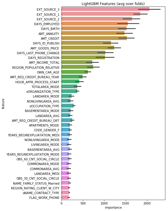
Feature importance
Appendix: meaning of each field
| field | Meaning |
|---|---|
| SK_ID_CURR | ID of this application |
| TARGET | Repayment risk of the applicant: 1-high risk; 0-low risk |
| NAME_CONTRACT_TYPE | Loan type: cash or revolving |
| CODE_GENDER | Applicant gender |
| FLAG_OWN_CAR | Does the applicant have a car |
| FLAG_OWN_REALTY | Does the applicant have a room |
| CNT_CHILDREN | Number of children of applicant |
| AMT_INCOME_TOTAL | Income status of applicants |
| AMT_CREDIT | Loan amount applied for this time |
| AMT_ANNUITY | Loan annuity |
| AMT_GOODS_PRICE | If it is a consumer loan, change the field to represent the actual price of the goods |
| NAME_TYPE_SUITE | Accompanying personnel of the applicant for this application |
| NAME_INCOME_TYPE | Type of applicant's income |
| NAME_EDUCATION_TYPE | Education level of applicant |
| NAME_FAMILY_STATUS | Applicant's marital status |
| NAME_HOUSING_TYPE | Living conditions of the applicant (rented house, purchased house, lived with parents, etc.) |
| REGION_POPULATION_RELATIVE | Population density of applicant's residence, standardized |
| DAYS_BIRTH | Applicant's date of birth (days from the date of application, negative) |
| DAYS_EMPLOYED | Working years of the applicant (days from the date of application, negative) |
| DAYS_REGISTRATION | The time when the applicant last modified the registration information (days from the date of application, negative value) |
| DAYS_ID_PUBLISH | The time when the applicant last modified the identity document of the loan application (days from the date of application, negative value) |
| FLAG_MOBIL | Does the applicant provide personal phone number (1-yes, 0-no) |
| FLAG_EMP_PHONE | Does the applicant provide home phone (1-yes, 0-no) |
| FLAG_WORK_PHONE | Does the applicant provide a work phone number (1-yes, 0-no) |
| FLAG_CONT_MOBILE | Whether the personal phone of the applicant can be dialed (1-yes, 0-no) |
| FLAG_EMAIL | Whether the applicant provides email (1-yes, 0-no) |
| OCCUPATION_TYPE | Position of applicant |
| REGION_RATING_CLIENT | The company's rating of the applicant's residential area (1, 2, 3) |
| REGION_RATING_CLIENT_W_CITY | In consideration of the city, the company's rating of the applicant's residential area (1,2,3) |
| WEEKDAY_APPR_PROCESS_START | What day of the week is the applicant initiating the application |
| HOUR_APPR_PROCESS_START | The hour the applicant initiated the application |
| REG_REGION_NOT_LIVE_REGION | Whether the permanent address and contact address provided by the applicant match (1-do not match, 2-match, regional level) |
| REG_REGION_NOT_WORK_REGION | Whether the permanent address and working address provided by the applicant match (1-mismatch, 2-match, region level) |
| LIVE_REGION_NOT_WORK_REGION | Whether the contact address and working address provided by the applicant match (1-do not match, 2-match, regional level) |
| REG_CITY_NOT_LIVE_CITY | Whether the permanent address and contact address provided by the applicant match (1-do not match, 2-match, city level) |
| REG_CITY_NOT_WORK_CITY | Whether the permanent address and working address provided by the applicant match (1-do not match, 2-match, city level) |
| LIVE_CITY_NOT_WORK_CITY | Whether the contact address and work address provided by the applicant match (1-do not match, 2-match, city level) |
| ORGANIZATION_TYPE | Organization type of applicant |
| EXT_SOURCE_1 | Standardized scoring of external data source 1 |
| EXT_SOURCE_2 | Standardized scoring of external data source 2 |
| EXT_SOURCE_3 | Standardized scoring of external data source 3 |
| APARTMENTS_AVG <----> EMERGENCYSTATE_MODE | Standardized scores of various indicators of the applicant's living environment |
| OBS_30_CNT_SOCIAL_CIRC LE <----> DEF_60_CNT_SOCIAL_CIRCLE | The meaning of these fields is not understood |
| DAYS_LAST_PHONE_CHANGE | Time when the applicant last modified the mobile phone number (days from the date of application, negative value) |
| FLAG_DOCUMENT_2 <----> FLAG_DOCUMENT_21 | Does the applicant provide additional documents 2, 3, 4.21 |
| AMT_REQ_CREDIT_BUREAU_HOUR | The number of times the applicant has been inquired about the credit investigation within 1 hour before the application is initiated |
| AMT_REQ_CREDIT_BUREAU_DAY | The number of times the applicant has been inquired about the credit investigation within one day before the application is initiated |
| AMT_REQ_CREDIT_BUREAU_WEEK | The number of times the applicant has been inquired about the credit investigation within one week before the application is initiated |
| AMT_REQ_CREDIT_BUREAU_MONTH | The number of times the applicant has been inquired about the credit investigation within one month before the application is initiated |
| AMT_REQ_CREDIT_BUREAU_QRT | The number of times the applicant has been inquired about the credit investigation within one quarter before the application is initiated |
| AMT_REQ_CREDIT_BUREAU_YEAR | The number of times the applicant has been inquired about the credit investigation within one year before the application is initiated |
From the table, we can roughly guess some information, such as: location, name, ncome and organization types should have strong linear correlation; days, last, phone, change, hour, appr, process, start and other information may not be important features; they can be verified in later feature analysis and take specific dimension reduction measures

