Analysis of python matrix multiplication (multiply / maumull / * / @)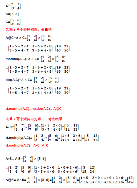

1. Load data

def load_data(path,transpose=True):
    data=sio.loadmat(path)
    y=data.get("y")#before reshape:(5000, 1)
    y=y.reshape(y.shape[0])
    X=data.get("X")#(5000,400),(400,)
    if transpose:
        #Vectorization, so that each column becomes a sample and each row is a sample?
        X=np.array([im.reshape((20,20)).T for im in X])
        X=np.array([im.reshape(400) for im in X])#Expand the sample to the original (400,)
    return X,y

X, y = load_data('code/ex3-neural network/ex3data1.mat')
print(X.shape)
print(y.shape)

(5000, 400)
(5000,)

2. drawing

def plot_an_image(image):
    fig,ax=plt.subplots(figsize=(1,1))
    ax.matshow(image.reshape((20, 20)), cmap=matplotlib.cm.binary)
    plt.xticks(np.array([]))  # Just get rid of marks
    plt.yticks(np.array([]))

pick_one = np.random.randint(0, 5000)
plot_an_image(X[pick_one,:])
plt.show()
print('this should be {}'.format(y[pick_one]))

• Maplotlib.pyplot.mattshow matrix visualization, plot a matrix or an array as an image.
• In matplotlib, ticks represent scale, and scale has two meanings, one is locks, the other is tick labels. In drawing, the x-axis and y-axis are continuous, so the marking can be specified at will, that is, to find the position on the continuous variable, and the scale label can be replaced correspondingly:
  xticks() returns two objects, one is the locks and the other is the scale labels
  locs, labels = xticks()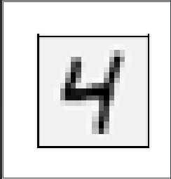
  

def plot_100_image(X):
    size=int(np.sqrt(X.shape[1]))
    sample_idx=np.random.choice(np.arange(X.shape[0]),100)#100 out of 5000 samples
    sample_images=X[sample_idx,:]
    fig,ax_array=plt.subplots(nrows=10,ncols=10,sharex=True,sharey=True)
    for r in range(10):
        for c in range(10):
            ax_array[r,c].matshow(sample_images[10*r+c].reshape((size,size)))
            plt.xticks(np.array([]))
            plt.yticks(np.array([]))  
            #Drawing function, drawing 100 pictures

• np.arange()
  The function returns a fixed step arrangement with an end point and a start point, such as [1,2,3,4,5]. The start point is 1, the end point is 5, and the step is 1.
  The number of parameters: NP. Range() function is divided into one parameter, two parameters, three parameters and three cases
  1) For a parameter, the parameter value is the end point, the start point is 0 by default, and the step length is 1 by default.
  2) When there are two parameters, the first parameter is the starting point, the second parameter is the end point, and the step length takes the default value of 1.
  3) For the three parameters, the first parameter is the starting point, the second parameter is the end point, and the third parameter is the step size. Where step size supports decimal
  Original link: https://blog.csdn.net/qq_41550480/article/details/89390579
• random.choice() randomly selects content: you can randomly select content from an int number or a 1-D array, and return the selection result in an n-D array.

Preparation data

raw_X, raw_y = load_data('code/ex3-neural network/ex3data1.mat')
print(raw_X.shape)
print(raw_y.shape)

(5000, 400)
(5000,)

# Add x0=1
X = np.insert(raw_X, 0, values=np.ones(raw_X.shape[0]), axis=1)#First column inserted (all 1)
X.shape

(5000, 401)
Vectorization label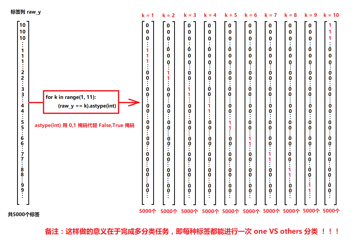

y_matrix=[]
for k in range(1,11):
    y_matrix.append((raw_y==k).astype(int))
# last one is k==10, it's digit 0, bring it to the first position
y_matrix = [y_matrix[-1]] + y_matrix[:-1]#Y matrix [- 1] is (5000,), [y matrix [- 1]] is (15000), y matrix [: - 1] shape is (95000)
y = np.array(y_matrix)
y.shape

(10, 5000)

Training one-dimensional model

def sigmoid(z):
    return 1 / (1 + np.exp(-z))

def cost(theta,X,y):
    return np.mean(-y * np.log(sigmoid(X @ theta)) - (1 - y) * np.log(1 - sigmoid(X @ theta)))

def regularized_cost(theta, X, y, lr=1):
    theta_ji_to_n=theta[1:]
    regularized_term=(lr/(2*len(X)))*np.sum(np.power(theta_ji_to_n,2))
    return cost(theta,X,y)+regularized_term

def gradient(theta, X, y):
    '''just 1 batch gradient'''
    return (1 / len(X)) * X.T@ (sigmoid(X @ theta) - y)

def regularized_gradient(theta, X, y, lr=1):
    theta_j1_to_n = theta[1:]
    regularized_theta = (lr / len(X)) * theta_j1_to_n
    regularized_term = np.concatenate([np.array([0]), regularized_theta])
    return gradient(theta, X, y) + regularized_term
    

def logistic_regression(X,y,lr=1):
    theta=np.zeros(X.shape[1])
    res=opt.minimize(fun=regularized_cost,x0=theta,args=(X,y,lr),method="TNC",jac=regularized_gradient, options={'disp': True})
    final_theta = res.x
    return final_theta

def predict(x, theta):
    prob = sigmoid(x @ theta)
    return (prob >= 0.5).astype(int)

t0=logistic_regression(X,y[0])
print(t0.shape)
y_pred = predict(X, t0)
print('Accuracy={}'.format(np.mean(y[0] == y_pred)))

(401,)
Accuracy=0.9974

• Numpy provides * * numpy.concatenate((a1,a2,...) ), axis=0) * * function. Can complete the splicing of multiple arrays at one time. Among them, a1,a2 Is an array type parameter

a=np.array([1,2,3])
b=np.array([11,22,33])
c=np.array([44,55,66])
np.concatenate((a,b,c),axis=0) # By default, axis=0 can be left blank
array([ 1, 2, 3, 11, 22, 33, 44, 55, 66]) #For one-dimensional array splicing, the value of axis does not affect the final result

Training multidimensional data

k_theta = np.array([logistic_regression(X, y[k]) for k in range(10)])
print(k_theta.shape)

(10, 401)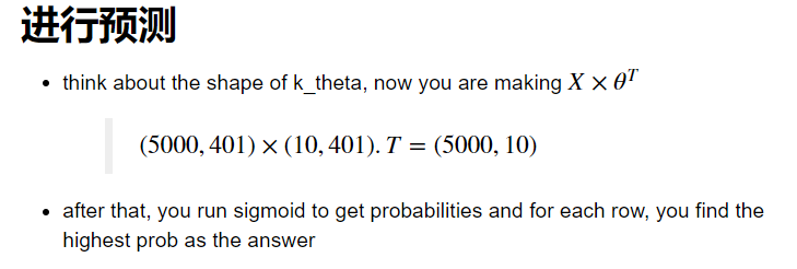

prob_matrix = sigmoid(X @ k_theta.T)
np.set_printoptions(suppress=True)
print(prob_matrix.shape)
print(prob_matrix)

(5000, 10)
[[0.99577353 0. 0.00053536 ... 0.0000647 0.00003916 0.00172426]
[0.99834639 0.0000001 0.00005611 ... 0.00009681 0.00000291 0.00008494]
[0.99139822 0. 0.00056824 ... 0.00000655 0.02655352 0.00197512]
...
[0.00000068 0.04144103 0.00321037 ... 0.00012724 0.00297365 0.707625 ]
[0.00001843 0.00000013 0.00000009 ... 0.00164807 0.0680994 0.86118731]
[0.02879745 0. 0.00012979 ... 0.36617606 0.00498225 0.14829291]]

y_pred=np.argmax(prob_matrix,axis=1)#Returns the index value of the maximum value of each row
print(y_pred)

[0 0 0 ... 9 9 7]

y_answer = raw_y.copy()
y_answer[y_answer==10] = 0
print(classification_report(y_answer, y_pred))

precision    recall  f1-score   support

      0       0.97      0.99      0.98       500
      1       0.95      0.99      0.97       500
      2       0.95      0.92      0.93       500
      3       0.95      0.91      0.93       500
      4       0.95      0.95      0.95       500
      5       0.92      0.92      0.92       500
      6       0.97      0.98      0.97       500
      7       0.95      0.95      0.95       500
      8       0.93      0.92      0.92       500
      9       0.92      0.92      0.92       500

avg / total 0.94 0.94 0.94 5000

Feedforward prediction of neural network

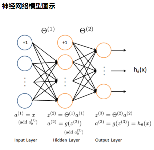
Next, we evaluate the model by loading the existing weights:

def load_weight(path):
    data=sio.loadmat(path)
    return data["Theta1"],data["Theta2"]

theta1, theta2 = load_weight('code/ex3-neural network/ex3weights.mat')

theta1.shape, theta2.shape

((25, 401), (10, 26))
Because in the data loading function, the original data is transposed, however, the transposed data is not compatible with the given parameters, because these parameters are trained by the original data. So in order to apply the given parameters, I need to use the raw data (not transpose)

X, y = load_data('code/ex3-neural network/ex3data1.mat',transpose=False)

X = np.insert(X, 0, values=np.ones(X.shape[0]), axis=1)  # intercept

print(X.shape)
print(y.shape)

(5000, 401)
(5000,)

feed forward prediction

First floor:

a1=X#input
z2=a1@theta1.T
z2.shape

(5000, 401)
(5000,)

The second floor:

z2 = np.insert(z2, 0, values=np.ones(z2.shape[0]), axis=1)#Add a column of bias
a2=sigmoid(z2)
a2.shape

(5000, 26)

z3=a2@theta2.T
a3=sigmoid(z3)
a3

array([[0.00013825, 0.0020554 , 0.00304012, ..., 0.00049102, 0.00774326,
0.99622946],
[0.00058776, 0.00285027, 0.00414688, ..., 0.00292311, 0.00235617,
0.99619667],
[0.00010868, 0.0038266 , 0.03058551, ..., 0.07514539, 0.0065704 ,
0.93586278],
...,
[0.06278247, 0.00450406, 0.03545109, ..., 0.0026367 , 0.68944816,
0.00002744],
[0.00101909, 0.00073436, 0.00037856, ..., 0.01456166, 0.97598976,
0.00023337],
[0.00005908, 0.00054172, 0.0000259 , ..., 0.00700508, 0.73281465,
0.09166961]])

y_pred = np.argmax(a3, axis=1) + 1  # numpy is 0 base index, +1 for matlab convention, returns the index of axis maximum value along the axis, axis=1 represents the row
y_pred.shape

print(classification_report(y, y_pred))

precision recall f1-score support

      1       0.97      0.98      0.97       500
      2       0.98      0.97      0.97       500
      3       0.98      0.96      0.97       500
      4       0.97      0.97      0.97       500
      5       0.98      0.98      0.98       500
      6       0.97      0.99      0.98       500
      7       0.98      0.97      0.97       500
      8       0.98      0.98      0.98       500
      9       0.97      0.96      0.96       500
     10       0.98      0.99      0.99       500

avg / total 0.98 0.98 0.98 5000