The rise of deep learning has brought us new efforts and trial directions, and also brought higher requirements for the computing power of machines. GPU acceleration is the key to improve computing speed, but for most people, buying a good video card is too expensive. If you are not a local tyrant, if you use a computer with extremely limited computing resources, if you want to train a deep learning neural network of your own and quickly iterate without spending money to upgrade your own machine, then you can refer to the following article.

Next, I'll show you how to use a broken set display notebook to build a deep learning model of your own using the cloud computing resources provided by Google, and how to save the training results to your own computer. This will allow you to put model iterations that require a lot of computing in the cloud, and model usage that requires less computing resources in the client, your own computer.

1. Visit Google

First of all, you need a tool that can access Google and find it yourself.

 

2. The use of Google cloud disk's colab notebook - Laboratory

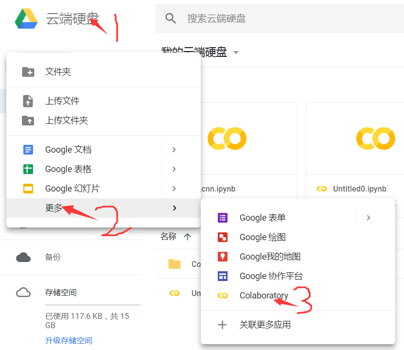
First, create a new laboratory:

 

Then, enter the notebook and make basic settings: file name, required software environment, whether to use GPU acceleration (this is the main purpose), etc.

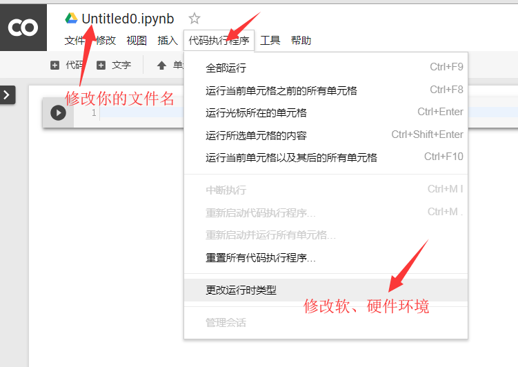
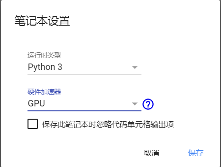
After clicking the "change runtime type" button, in the pop-up dialog box, set the type of software and hardware you need. Here I set it as: Python 3, use GPU acceleration.

 

After the above steps, you can use free cloud computing resources, in which you can try to upload and download files, import various toolkits, write your own code and run it.

3. Use of code snippets

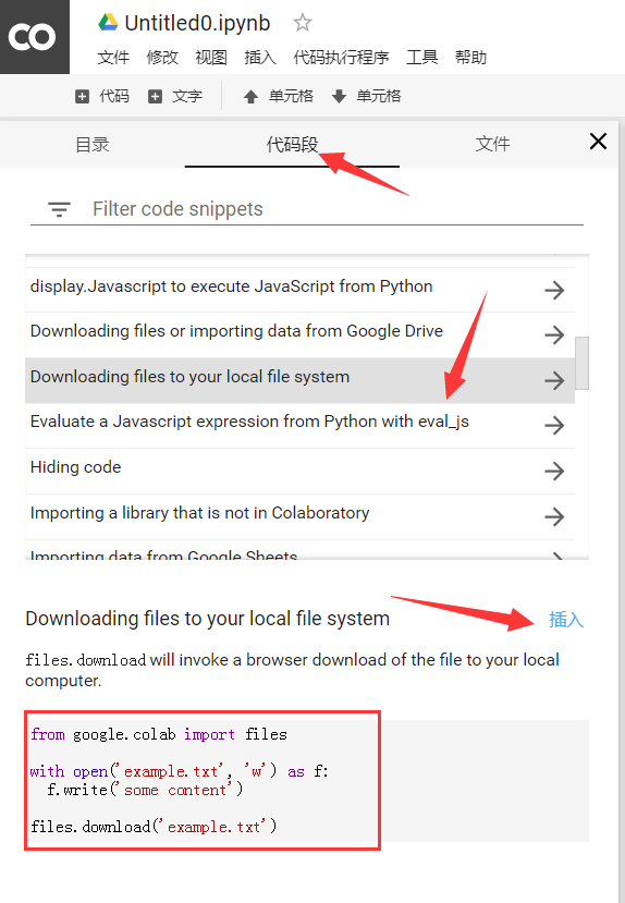
When entering the notebook, its basic use is similar to that of Jupyter Notebook, with similar interface and basic operation. In addition, it also provides various ready-made snacks -- code snippets: click the hidden window on the right, and you can see three options: directory, code snippet and file. The middle code snippet provides us with various practical and small function examples, which we can check Look at the small features and try to use them to address specific needs.

The following figure shows the steps to use. An example is a code snippet to save the file to the local computer. There are other functions that you can use on demand.

4. A complete example

Through the above steps, everyone can do something according to their own ideas. Here's an example of me. It's a complete process of building a CNN handwritten font recognition network and online iterative training, then saving the model on the server assigned to us by Google, and finally downloading the saved model to your own computer.

First, the code related to CNN network construction, training, testing and model preservation:

# -*- coding: utf-8 -*-
"""
Created on Wed Oct 24 09:48:06 2018

@author: Leon

//Content:
//Taking LeNet-5 network as a model, CNN is built to train and test mnist handwritten numbers
//Add name to the key sensor to facilitate the call after saving the model
"""

import tensorflow.examples.tutorials.mnist.input_data as input_data
import tensorflow as tf
import time
tf.reset_default_graph()#If there is an error in saving the model, clear the existing diagram
mnist = input_data.read_data_sets("MNIST_data/",one_hot=True)

x = tf.placeholder(tf.float32,[None,784],name='x')
y = tf.placeholder(tf.float32,[None,10],name='y')

def weight_variable(shape,name):  
    initial = tf.truncated_normal(shape, stddev = 0.1,name=name) # Truncated normal distribution  
    return tf.Variable(initial)  
  
def bias_variable(shape,name):  
    initial = tf.constant(0.1, shape=shape, name=name) # Constant 0.1  
    return tf.Variable(initial)

# =============================================================================
#  First layer: convolution + activation + pooling
# =============================================================================
# Convolution kernel 5 * 5, channel 1, number 32
filter1 = weight_variable([5,5,1,32],name='filter1')
# Convolution layer: Step 1 * 1,
# Padding has two parameters:
# SAME -- output size is: input size / s;
# VALID -- output size is: (input size - f+1)/s
x_img = tf.reshape(x,[-1,28,28,1],name='x_img')
conv1 = tf.nn.conv2d(x_img, filter1, strides=[1,1,1,1], padding='SAME',name='conv1')
# Activate layer: add offset, then activate
bias1 = bias_variable([32],name='bias1')
relu1 = tf.nn.relu(conv1+bias1,name='relu1')
# Pool layer: window size 2 * 2, step size 2 * 2
pool1 = tf.nn.max_pool(relu1,ksize=[1,2,2,1],strides=[1,2,2,1],padding='SAME',name='pool1')
print("First floor output size:",pool1.shape)

# =============================================================================
# The second layer: convolution + activation + pooling
# =============================================================================
# Convolution kernel size 5 * 5, 1 channel, 64 convolution kernels
filter2 = weight_variable([5,5,32,64],name='filter2')
# Convolution layer: Step 1 * 1
conv2 = tf.nn.conv2d(pool1,filter2,strides=[1,1,1,1],padding='SAME',name='conv2')
# Activate layer: add offset, then activate
bias2 = bias_variable([64],name='bias2')
relu2 = tf.nn.relu(conv2+bias2,name='relu2')
# Pooled layer:
pool2 = tf.nn.max_pool(relu2,ksize=[1,2,2,1],strides=[1,2,2,1],padding='SAME',name='pool2')
print("Output size of the second layer:", pool2.shape)

# =============================================================================
# The third layer: full connection layer
# =============================================================================
# Extract the size of the output of the previous layer
shape = pool2.shape.as_list()
# Stretch the upper layer output to construct the layer input
fc_input = tf.reshape(pool2,[-1,shape[1]*shape[2]*shape[3]])
# Weight of full connection layer: the size is the number of input * neurons in this layer, i.e., the following: [shape[1]*shape[2]*shape[3],32]
fc_w = weight_variable([shape[1]*shape[2]*shape[3],1024], name='fc_w')
# Migration of all connected layer: the size is the number of neurons in this layer-32
fc_b = bias_variable([1024],name='fc_b')
# Establish full connection structure of this layer and activate
fc_out = tf.nn.relu(tf.matmul(fc_input,fc_w)+fc_b,name='fc_out')
print("Output size of the third layer:", fc_out.shape)

# Dropout to prevent over fitting  
# Before the output layer, dropout is turned on during training and off during testing  
keep_prob = tf.placeholder(tf.float32,name='keep_prob')
fc_out_drop = tf.nn.dropout(fc_out, keep_prob,name='fc_out_drop')

# =============================================================================
# Output layer
# =============================================================================
out_w = weight_variable([1024,10],name='out_w')
out_b = bias_variable([10],name='out_b')
pred = tf.nn.softmax(tf.matmul(fc_out_drop,out_w)+out_b,name='pred')

# Define loss function
loss = -tf.reduce_sum(y*tf.log(pred),name='loss')
# Define optimizer: Adam optimization function
optimizer = tf.train.AdamOptimizer(learning_rate=0.001,name='optimizer').minimize(loss)

# Define evaluation indicators - accuracy rate
bool_pred = tf.equal(tf.arg_max(y,1), tf.arg_max(pred,1))
accuracy = tf.reduce_mean(tf.cast(bool_pred,tf.float32),name='accuracy')

# Define global variable initialization
init = tf.global_variables_initializer()

# Define save model class
saver = tf.train.Saver()

# Startup diagram
with tf.Session() as sess:
    # Execution is initialization
    sess.run(init)
    # The total number of batch es in the training sample
    total_batch_nums = int(mnist.train.num_examples/50)
    for epoch in range(1):
        avg_loss = 0.
        time_start = time.clock()
        for i in range(total_batch_nums):
            
            batch = mnist.train.next_batch(50)
            batch_xs,batch_ys = batch
#            batch_xs = batch_xs.reshape([-1,28,28,1])
            sess.run(optimizer,feed_dict={x:batch_xs,y:batch_ys,keep_prob:0.5})
#            avg_loss += sess.run(loss, feed_dict={x:batch_xs,y:batch_ys})
        time_end = time.clock()
        
        if epoch %1 == 0:
            accuracy_eval = sess.run(accuracy, 
                                     feed_dict={x:batch_xs,y:batch_ys,keep_prob:1.0})
            print("Epoch:","%04d"%(epoch+1),
#                  "loss:","%.4f"%avg_loss,
                  "accuracy:",accuracy_eval,
                  "running time:","%g"%(time_end-time_start))
            
    saver.save(sess,'model/my_model')
    accuracy_test = sess.run(accuracy,feed_dict={x:mnist.test.images,y:mnist.test.labels,keep_prob:1.0})
    print("test accuracy:",accuracy_test)

Add a digression: the temporary server assigned by the registry to us is based on the Linux environment. We can also interact with the system in this Notebook, but we need to add "!" before the Linux command For example,

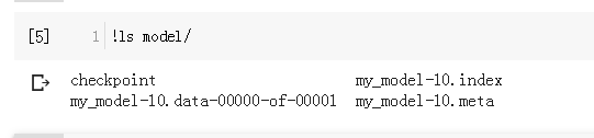
Because my code above is to save the model in a subdirectory "model" of the current directory, so by command:! ls model / lists all the files in the directory.

OK, then we can download these files. Here is the code to download the saved model to the local:

# Download saved model to local
import os
from google.colab import files

dir_list = os.listdir("model")
for file in dir_list:
  path = 'model/'+file
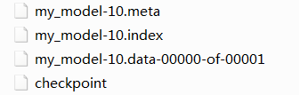
  files.download(path)

By executing the above code, you can find the model you just saved in the download directory of your browser, namely the following four files:

Finally, we will download the local model and apply it on our own computer:

# -*- coding: utf-8 -*-
"""
Created on Wed Oct 31 10:53:16 2018

@author: Leon

//Content:
1,From the saved model, load the previously trained CNN network
2,Using the names of variables in the network“ name"To extract the corresponding variables
3,For related variables feed，structure feed_dict
4,Finally, the model is used to test the new data
"""

import tensorflow as tf
import tensorflow.examples.tutorials.mnist.input_data as input_data
mnist = input_data.read_data_sets("MNIST_data/",one_hot=True)


with tf.Session() as sess:
    saver = tf.train.import_meta_graph("model/my_model.meta")
    saver.restore(sess,tf.train.latest_checkpoint("model/"))
    
    graph = tf.get_default_graph()
    x = graph.get_tensor_by_name("x:0")
    y = graph.get_tensor_by_name("y:0")
    keep_prob = graph.get_tensor_by_name("keep_prob:0")
    accuracy = graph.get_tensor_by_name("accuracy:0")
    
    accuracy_eval = sess.run(accuracy, feed_dict={x:mnist.test.images[:1000],y:mnist.test.labels[:1000],keep_prob:1.0})
    print("acc:",accuracy_eval)

OK, it's done! So far, we have completed the whole process from using Google cloud computing resources to train our own model, to transplanting the model to other machines for testing and application, avoiding the problem of too long iteration time caused by insufficient computing power.