Recently, I read the article "a dynamic clustering approach to data driven assessment personalization" on Management Science, in which I mentioned a multiarmed bandit model. I want to study it in depth, but when I check various websites, there is no introduction about this problem in Chinese, so I go to the tubing to learn it, and then translate it into Chinese to share with you here.

Exploration and esploitation tradeoff

There is a classic problem in reinforcement learning, that is, exploration and deployment tradeoff. There is a dilemma in this problem: should we spend our energy to explore so as to have a more accurate estimate of income, or should we choose the action with the expectation of maximum income according to the information we have at present?
The multiarmed bandit model is extended

Multiarmed-Bandit Model

Suppose there are n slot machines now, and the revenue of each slot machine is different, but we don't know the expected revenue of each slot machine in advance.
We assume here that the revenue of each slot machine follows a normal distribution with variance of 1, and the mean value is not known in advance. We need to explore the revenue distribution of each slot machine, and finally let the action choose the slot machine with the most expected revenue.

Traditional solution A/B test

The idea of A/B test is to assign the same number of tests to each slot machine, and then select the slot machine with the best performance for all the remaining operations according to the test results of all slot machines.
The biggest disadvantage of this method is to separate exploration from development. In the process of exploration, we only consider exploration and collect information, but in the stage of development, we don't think about exploration any more, so we lose the chance of learning. We may fall into the local optimum, and we can't find the optimal slot machine.

Epsilon grey algorithm

Epsilon greedy algorithm is also a greedy algorithm, but in the process of each selection, it will choose other actions that are not the optimal actions with a small change, so it can continue to explore. Because epsilon is less and the algorithm will find the best action, the probability of choosing the best action will approach to 1-epsilon.
Here's the python code:

import numpy as np
import matplotlib.pyplot as plt


class EpsilonGreedy:
    def __init__(self):
        self.epsilon = 0.1  # Set epsilon value
        self.num_arm = 10  # Set the number of arm s
        self.arms = np.random.uniform(0, 1, self.num_arm)  # Set the average value of each arm as a random number between 0-1
        self.best = np.argmax(self.arms)  # Find the index of the best arm
        self.T = 50000  # Set the number of actions to take
        self.hit = np.zeros(self.T)  # It is used to record whether the optimal arm is found for each action
        self.reward = np.zeros(self.num_arm)  # Used to record the average revenue of each arm after each action
        self.num = np.zeros(self.num_arm)  # Used to record the total number of times each arm is pulled after each action

    def get_reward(self, i):  # i is the index of arm
        return self.arms[i] + np.random.normal(0, 1)  # The generated revenue is the average value of arm plus a fluctuation

    def update(self, i):
        self.num[i] += 1
        self.reward[i] = (self.reward[i]*(self.num[i]-1)+self.get_reward(i))/self.num[i]

    def calculate(self):
        for i in range(self.T):
            if np.random.random() > self.epsilon:
                index = np.argmax(self.reward)
            else:
                a = np.argmax(self.reward)
                index = a
                while index == a:
                    index = np.random.randint(0, self.num_arm)
            if index == self.best:
                self.hit[i] = 1  # If the obtained arm is the optimal arm, record it as 1
            self.update(index)

    def plot(self):  # Drawing view convergence
        x = np.array(range(self.T))
        y1 = np.zeros(self.T)
        t = 0
        for i in range(self.T):
            t += self.hit[i]
            y1[i] = t/(i+1)
        y2 = np.ones(self.T)*(1-self.epsilon)
        plt.plot(x, y1)
        plt.plot(x, y2)
        plt.show()


E = EpsilonGreedy()
E.calculate()
E.plot()

The final results are as follows: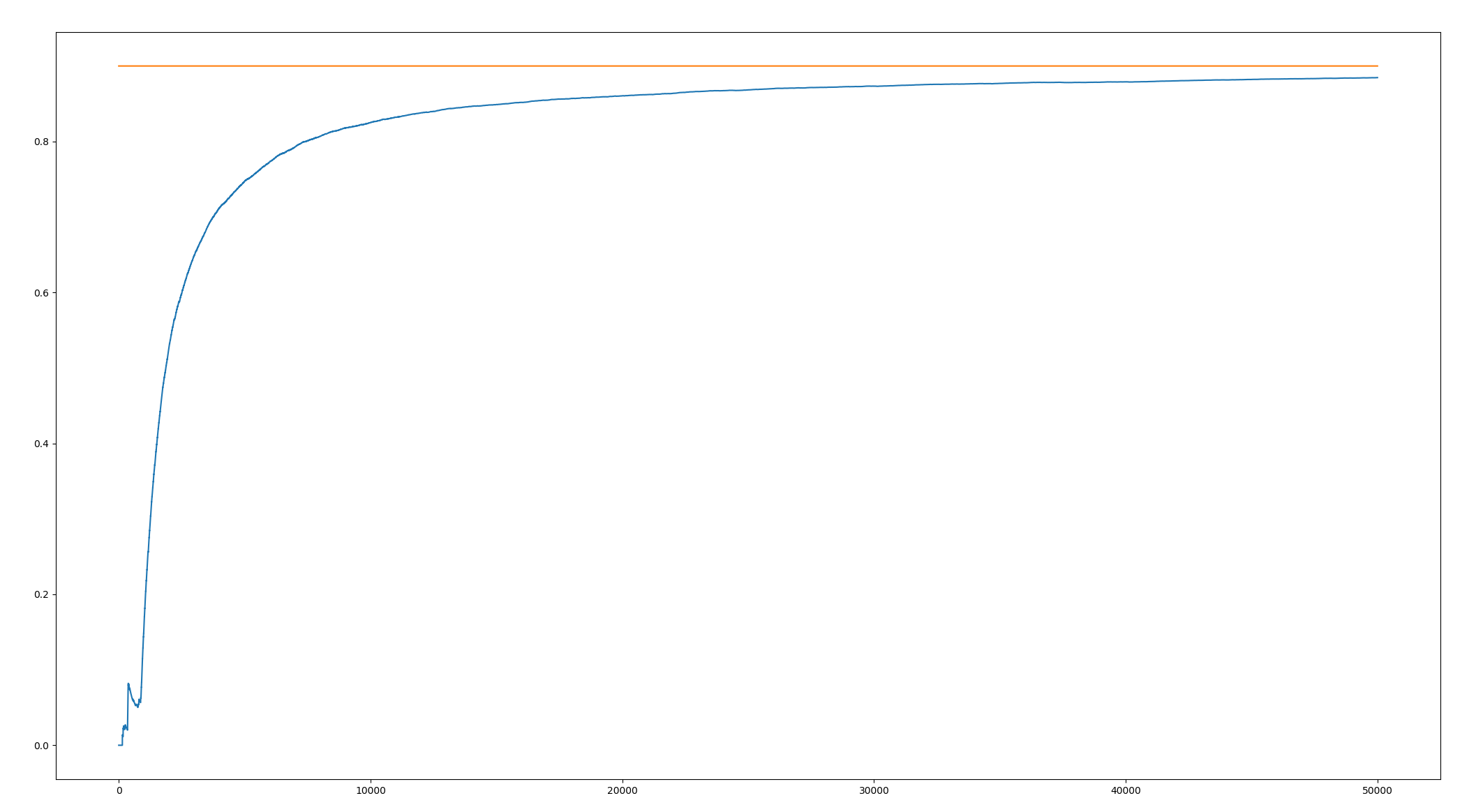

With the continuous action, the cumulative accuracy (the frequency of selecting the optimal arm) is rising, and it approaches the online 1 ϵϵϵϵϵϵϵϵϵϵϵϵϵϵϵϵϵϵϵϵϵϵϵϵϵϵ!