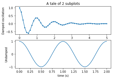
Drawing 2D chart on jupyter notebook

%matplotlib inline #Inline display
# %config InlineBackend.figure_format="svg" #Display on Web page in svg format
import numpy as np
import matplotlib.pyplot as plt

x1 = np.linspace(0.0, 5.0)
x2 = np.linspace(0.0, 2.0)

y1 = np.cos(2 * np.pi * x1) * np.exp(-x1)
y2 = np.cos(2 * np.pi * x2)

plt.subplot(2, 1, 1)
plt.plot(x1, y1, '.-')
plt.title('A tale of 2 subplots')
plt.ylabel('Damped oscillation')

plt.subplot(2, 1, 2)
plt.plot(x2, y2, '-')
plt.xlabel('time (s)')
plt.ylabel('Undamped')

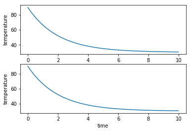
As the most basic differential equation, Newton's cooling law is used to demonstrate the first example

T′(t)=−α(T(t)−H)T(t)=H+(T0−H)e−αtT′(t)=−α(T(t)−H)T(t)=H+(T0−H)e−αt

%matplotlib inline 
from scipy.integrate import odeint
import matplotlib.pyplot as plt
import numpy as np

from IPython import display

# Differential equation of cooling law
def cooling_law_equ(w, t, a, H):
    return -1 * a * (w - H)

# The function of temp erature obtained by cooling law with respect to time t
def cooling_law_func(t, a, H, T0):
    return H + (T0 - H) * np.e ** (-a * t)

t = np.arange(0, 10, 0.01)
initial_temp = (90) #initial temperature
temp = odeint(cooling_law_equ, initial_temp, t, args=(0.5, 30)) #Cooling coefficient and ambient temperature
temp1 = cooling_law_func(t, 0.5, 30, initial_temp) #Comparison between the derived function and the result of scipy calculation
plt.subplot(2, 1, 1)
plt.plot(t, temp)
plt.ylabel("temperature")

plt.subplot(2, 1, 2)
plt.plot(t, temp1)
plt.xlabel("time")
plt.ylabel("temperature")

display.Latex("Newton's law of cooling $T'(t)=-a(T(t)- H)$)(Upper) sum $T(t)=H+(T_0-H)e^{-at}$(Next)")

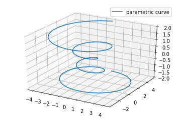
Drawing 3D charts on jupyter notebook

%matplotlib inline 
import matplotlib as mpl
from mpl_toolkits.mplot3d import Axes3D
import numpy as np
import matplotlib.pyplot as plt

mpl.rcParams['legend.fontsize'] = 10

fig = plt.figure()
ax = fig.gca(projection='3d')
theta = np.linspace(-4 * np.pi, 4 * np.pi, 100)
z = np.linspace(-2, 2, 100)
r = z**2 + 1
x = r * np.sin(theta)
y = r * np.cos(theta)
ax.plot(x, y, z, label='parametric curve')
ax.legend()

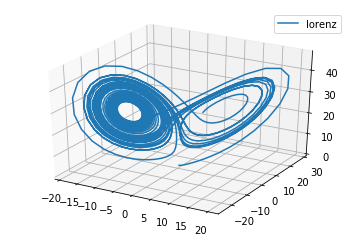
Demonstration of Lorentz attractor in three dimensional space

dxdt=σ⋅(y−x)dydt=x⋅(ρ−z)−ydzdt=xy−βzdxdt=σ⋅(y−x)dydt=x⋅(ρ−z)−ydzdt=xy−βz 

%matplotlib inline 
from scipy.integrate import odeint
import matplotlib as mpl
from mpl_toolkits.mplot3d import Axes3D
import numpy as np
import matplotlib.pyplot as plt

from IPython import display

fig = plt.figure()
ax = fig.gca(projection='3d')

def lorenz(w, t, p, r, b):
    # Position vector w, three parameters p, r, b
    x, y ,z = w.tolist()
    # Calculate dx/dt, dy/dt, dz/dt respectively
    return p * (y-x), x*(r-z)-y, x*y-b*z

t = np.arange(0, 30, 0.02)
initial_val = (0.0, 1.00, 0.0)

track = odeint(lorenz, initial_val, t, args=(10.0, 28.0, 3.0))
X, Y, Z = track[:,0], track[:,1], track[:,2]
ax.plot(X, Y, Z, label='lorenz')
ax.legend()

display.Latex(r"$\frac{dx}{dt}=\sigma\cdot(y-x) \\ \frac{dy}{dt}=x\cdot(\rho-z)-y \\ \frac{dz}{dt}=xy-\beta z$")

Copyright notice: This is the original article of the blogger. It can't be reproduced without the permission of the blogger. https://blog.csdn.net/m454078356/article/details/77776092

Article label: python

Personal classification: Python

Related hot words: python3∑ python3 python3 and python3 package python3 Library