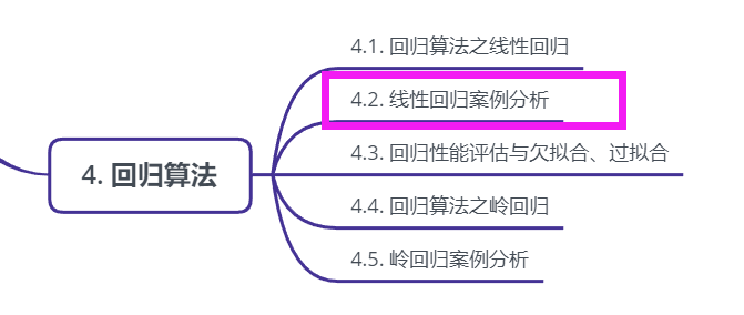
Article directory
4.2. Linear regression case analysis

Linear regression case analysis
Boston house price forecast
The regression model built in scikit learn is used to predict the "Boston house price" data. Some competition data can be obtained from the official website of kaggle, https://www.kaggle.com/datasets
1. Data description of housing prices in Boston
from sklearn.datasets import load_boston

boston = load_boston()

print boston.DESCR
2. Boston area housing price data segmentation
from sklearn.cross_validation import train_test_split
import numpy as np
X = boston.data
y = boston.target

X_train,X_test,y_train,y_test = train_test_split(X,y,random_state=33,test_size = 0.25)
3. Standardized processing of training and test data
from sklearn.preprocessing import StandardScaler
ss_X = StandardScaler()
ss_y = StandardScaler()

X_train = ss_X.fit_transform(X_train)
X_test = ss_X.transform(X_test)
y_train = ss_X.fit_transform(y_train)
X_train = ss_X.transform(y_test)
4. Using the simplest linear regression model, linear regression and gradient decline to estimate sgdregger to predict house prices
from sklearn.linear_model import LinearRegression
lr = LinearRegression()
lr.fit(X_train,y_train)
lr_y_predict = lr.predict(X_test)

from sklearn.linear_model import SGDRegressor
sgdr = SGDRegressor()
sgdr.fit(X_train,y_train)
sgdr_y_predict = sgdr.predict(X_test)
5. Performance evaluation
For different types of prediction, we can not strictly require that the numerical results of regression prediction should be strictly the same as the real values. In general, we want to measure the difference between the predicted value and the real value. Therefore, the evaluation function can be used for evaluation. Among them, the most intuitive evaluation index, mean squared error (MSE), is the objective of linear regression model optimization.
The calculation method of MSE is as follows:
{MSE=}\frac{1}{m}\sum_{i=1}{m}\left({y{i}-\bar{y}}\right)^{2}MSE=m1∑i=1m(y**i−y¯)2
Using MSE evaluation mechanism to evaluate the regression performance of the two models
from sklearn.metrics import mean_squared_error

print 'The mean square error of linear regression model is:',mean_squared_error(ss_y.inverse_transform(y_test),ss_y.inverse_tranform(lr_y_predict))
print 'The mean square error of gradient descent model is:',mean_squared_error(ss_y.inverse_transform(y_test),ss_y.inverse_tranform(sgdr_y_predict))
Through this comparison, it is found that the performance of the gradient descent estimation method is not as good as that of the linear regression method, but if the training data scale is very large, then the gradient method is very efficient in both classification and regression problems, which can save a lot of computing time without losing too much performance. According to the proposal of scikit learn optical network, if the data scale is more than 100000, the random gradient method is recommended to estimate the parameter model.
Note: linear regression is the simplest and most easy to use regression model. Because of the linear hypothesis between the feature and the regression target, it also limits its application scope to some extent. In particular, the vast majority of real-life case data can not guarantee strict linear relationship between various characteristics and regression objectives. However, we can still use linear regression model as the baseline system for most data analysis without knowing the relationship between features.
The complete code is as follows:
from sklearn.linear_model import LinearRegression, SGDRegressor, Ridge
from sklearn.preprocessing import StandardScaler
from sklearn.datasets import load_boston
from sklearn.cross_validation import train_test_split
from sklearn.metrics import mean_squared_error,classification_report
from sklearn.cluster import KMeans


def linearmodel():
    """
    //Linear regression for Boston dataset processing
    :return: None
    """

    # 1. Load dataset

    ld = load_boston()

    x_train,x_test,y_train,y_test = train_test_split(ld.data,ld.target,test_size=0.25)

    # 2. Standardized treatment

    # Eigenvalue processing
    std_x = StandardScaler()
    x_train = std_x.fit_transform(x_train)
    x_test = std_x.transform(x_test)


    # Target value processing

    std_y  = StandardScaler()
    y_train = std_y.fit_transform(y_train)
    y_test = std_y.transform(y_test)

    # 3. Estimator process

    # LinearRegression
    lr = LinearRegression()

    lr.fit(x_train,y_train)

    # print(lr.coef_)

    y_lr_predict = lr.predict(x_test)

    y_lr_predict = std_y.inverse_transform(y_lr_predict)

    print("Lr Predicted value:",y_lr_predict)


    # SGDRegressor
    sgd = SGDRegressor()

    sgd.fit(x_train,y_train)

    # print(sgd.coef_)

    y_sgd_predict = sgd.predict(x_test)

    y_sgd_predict = std_y.inverse_transform(y_sgd_predict)

    print("SGD Predicted value:",y_sgd_predict)

    # Ridge regression with regularization

    rd = Ridge(alpha=0.01)

    rd.fit(x_train,y_train)

    y_rd_predict = rd.predict(x_test)

    y_rd_predict = std_y.inverse_transform(y_rd_predict)

    print(rd.coef_)

    # Evaluation results of two models

    print("lr The mean square error of is:",mean_squared_error(std_y.inverse_transform(y_test),y_lr_predict))

    print("SGD The mean square error of is:",mean_squared_error(std_y.inverse_transform(y_test),y_sgd_predict))

    print("Ridge The mean square error of is:",mean_squared_error(std_y.inverse_transform(y_test),y_rd_predict))

    return None

