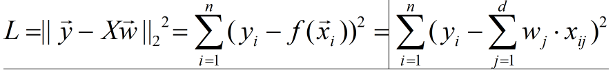
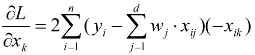
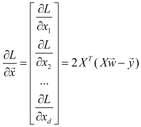
In this paper, the least square method is realized by the matrix realization form of the least square method and the for loop traversal form respectively, in which the BFGS algorithm is used in the parameter learning process.

(1) through matrix implementation, the code is as follows:

import numpy as np
import scipy.optimize as opt
import matplotlib.pyplot as plt

points = []
shape = []
np.random.seed(1)

# objective function
def obj_fun(theta, x, y_):
    theta = theta.reshape(3, 3)
    pre_dis = np.dot(x, theta)
    loss = np.sum((pre_dis - y_)**2) / 2
    points.append(loss)
    return loss

def prime(theta, x, y_):
    theta = theta.reshape(3, 3)
    pre_dis = np.dot(x, theta)
    print(pre_dis.shape)
    gradient = np.dot(np.transpose(x), (pre_dis - y_))
    return np.ravel(gradient)   # Expand two-dimensional matrix into one-dimensional vector

if __name__ == "__main__":
    feature = np.array([[1, 2, 3], [4, 5, 6], [7, 8, 9], [1, 5, 9]])
    dis_ = np.array([[0.1, 0.3, 0.6], [0.2, 0.4, 0.4], [0.3, 0.2, 0.5], [0.1, 0.3, 0.6]])
    #init_theta = np.ones([3, 3])
    init_theta = np.random.normal(size=(3, 3))
    shape = init_theta.shape
    print(prime(init_theta, x=feature, y_=dis_))


    #result = opt.fmin_l_bfgs_b(obj_fun2, init_theta, prime3, args=(feature, dis_, shape))
    result = opt.fmin_l_bfgs_b(obj_fun, init_theta, prime, args=(feature, dis_))
    # Note that when Fmin ﹣ BFGS ﹣ B algorithm is used, the optimized parameters are in result[0], and other algorithms are in result
    m_theta = np.array(result[0]).reshape(3, 3)
    print(np.dot(feature, m_theta))
    print(obj_fun(m_theta, feature, dis_))

    plt.plot(np.arange(len(points)), points)
    plt.show()

(2) through for loop traversal, the code is as follows:

import numpy as np
import scipy.optimize as opt
import matplotlib.pyplot as plt

points = []
shape = []
np.random.seed(1)

def obj_fun(theta, x, y_, theta_shape):
    (cols, rows) = theta_shape
    theta = theta.reshape([cols, rows])
    loss = 0
    for i in range(rows):
        pre_dis = per_obj_func(theta[:, i], x, y_[:, i])
        loss += pre_dis
    points.append(loss)
    return loss

#Calculation of one-dimensional objective function
def per_obj_func(theta, x, y_):
    loss = 0
    for i in range(len(x)):
        y = 0
        for j in range(len(theta)):
            y += theta[j] * x[i][j]
        loss += (y - y_[i])**2/2
    return loss

def prime(theta, x, y_, theta_shape):
    lst = []
    (cols, rows) = theta_shape
    theta = theta.reshape([cols, rows])
    for i in range(rows):
        per_lst = per_prime(theta[:, i], x, y_[:, i])
        lst.append(per_lst)
    np_lst = np.transpose(np.array(lst))
    return np.ravel(np_lst)

#Calculation of one-dimensional W partial derivative
def per_prime(theta, x, y_):
    lst = []
    for j in range(len(theta)):
        pre_dis = 0
        for i in range(len(x)):
            y = 0
            for k in range(len(x[0])):
                y += x[i][k] * theta[k]
            pre_dis += (y - y_[i]) * x[i][j]
        lst.append(pre_dis)
    return lst

if __name__ == "__main__":
    feature = np.array([[1, 2, 3], [4, 5, 6], [7, 8, 9], [1, 5, 9]])
    dis_ = np.array([[0.1, 0.3, 0.6], [0.2, 0.4, 0.4], [0.3, 0.2, 0.5], [0.1, 0.3, 0.6]])
    #init_theta = np.ones([3, 3])
    init_theta = np.random.normal(size=(3, 3))
    shape = init_theta.shape

    result = opt.fmin_l_bfgs_b(obj_fun, init_theta, prime, args=(feature, dis_, shape))
    # Note that when Fmin ﹣ BFGS ﹣ B algorithm is used, the optimized parameters are in result[0], and other algorithms are in result
    m_theta = np.array(result[0]).reshape(3, 3)
    print(np.dot(feature, m_theta))
    print(obj_fun(m_theta, feature, dis_, shape))
    plt.plot(np.arange(len(points)), points)
    plt.show()

Program running results:

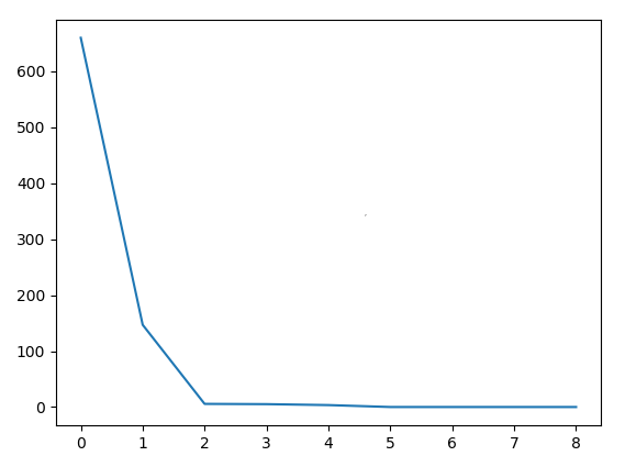
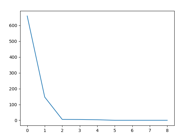
As you can see, the loss drop graph is the same, so the implementation is correct.

Be careful:

1. Here the shape is passed to the function because the opt.fmin ﹣ BFGS ﹣ B function changes the parameter of init ﹣ theta from (3,3) to (9,1), so

We need to reorganize W into the form of (3,3) within the function.

Note that the args of opt.fmin ﹣ BFGS ﹣ B needs to be used in both the fun function and the fprime function, so the parameter format needs to be unified, and two functions are not allowed

Inconsistent parameters for.

Because I compare dishes, so in the way of traversal, the W matrix is divided into several 3 X 1 single column matrices, so that the probability of error can be reduced.

Reference matrix method document:

https://blog.csdn.net/Ce1estial/article/details/77893760