Histogram equalization, as the name implies, deals with the distribution of image gray on statistical histogram, and is an image enhancement algorithm. The balanced gray value is the product of the probability of distribution of a certain gray value and the probability of distribution of all values lower than the value p and all gray levels L of the image.

Histogram equalization formula:

Take histogram equalization of 8-bit gray-scale image as an example, the first step is to count the probability of distribution of all gray-scale values of the image between 0 and 255; the second step is to calculate the corresponding value by accumulating the probability p(i) of each gray-scale level from low to high, and generate a look-up table; the third part is to generate a graph after the direct square equalization through the corresponding look-up table of the original image.

Statistical probability distribution and direct equilibrium calculation:

private Map<Integer, Double> getPDF(BufferedImage image) {
		Map<Integer, Double> map = new HashMap<>();
		int width = image.getWidth();
		int height = image.getHeight();
		double totalPixel = 3 * width * height;
		for (int i = 0; i < 256; i++) {
			map.put(i, 0.0);// Through the loop, fill 0-255 positions into the set, and the initial value is 0.
		}
		//Respectively count the total number of distribution on the image from 0 to 255
		for (int i = 0; i < image.getWidth(); i++) {
			for (int j = 0; j < image.getHeight(); j++) {
				int rgb = image.getRGB(i, j);
				int r = (rgb >> 16) & 0xff;
				int g = (rgb >> 8) & 0xff;
				int b = rgb & 0xff;
				map.put(r, map.get(r) + 1);
				map.put(g, map.get(g) + 1);
				map.put(b, map.get(b) + 1);
			}
		}
//Direct square equilibrium calculation to generate lookup table:
private void getTable(Map<Integer, Double> map) {
		double param = 0.0;
		for(int i = 0;i < 256;i++) {
			param += map.get(i);
			table[i] = (int)Math.round(param * 255);
		}
	}

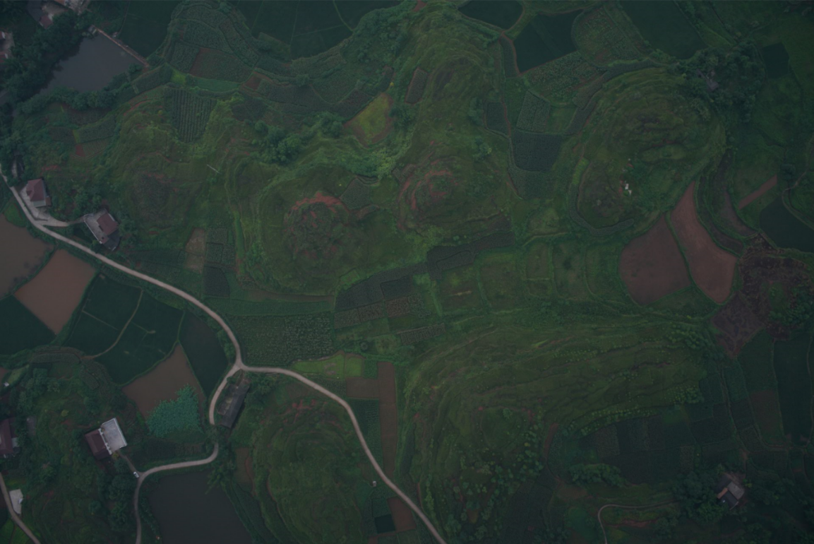
Test image:

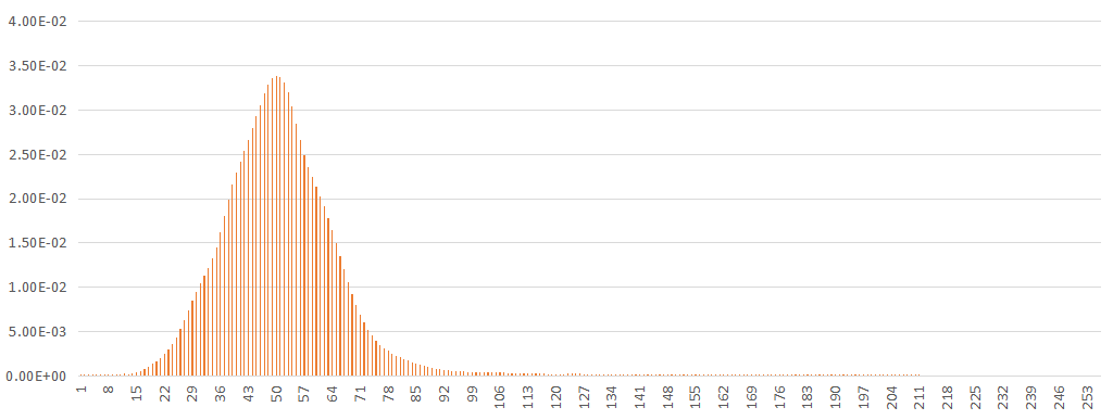
Histogram of distribution probability:

After direct equilibrium:

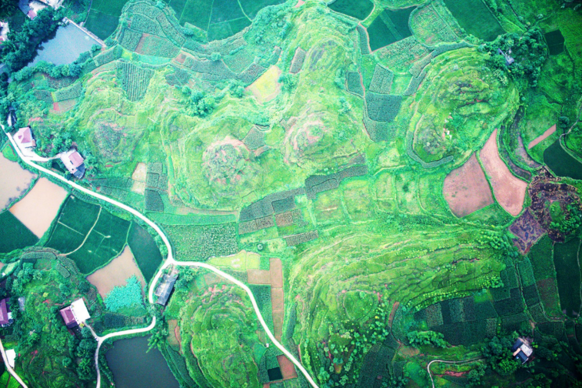
Probability distribution after direct equilibrium:

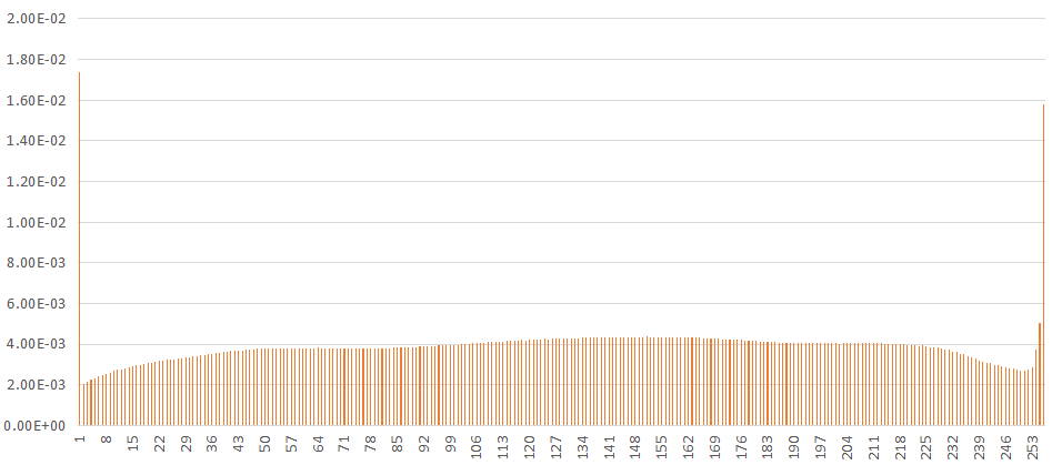
From the distribution of image and probability histogram, the gray peak value of the original image is about 50, and most of them are distributed on the smaller gray value. After histogram equalization, the image becomes bright, and the gray value is evenly distributed from 0 to 255. This is a traditional histogram equalization method, but it has some defects. Because the middle part of gray occupies a smaller probability distribution, it may be submerged by the gray near it with a larger probability. For example, if the statistical probability of gray value 100 is 50%, then the value after equalization is 128, and the probability distribution of 110 points is 50.1%, then the value after equalization calculation is still 128, and the gray value between 100 and 110 in the original image is also submerged. This problem can also be found in the test image details, as follows:

Details of the original part:

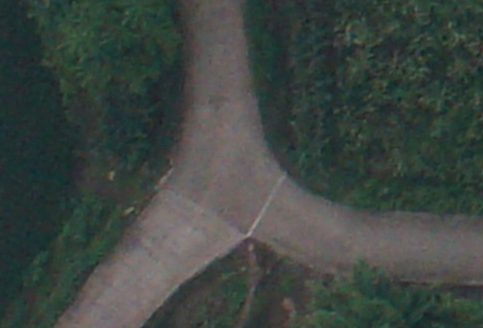
From the image, it can be seen that there is a boundary line formed by the obvious brightness difference at the three-way intersection. Then look at the details of the image after the square equalization.

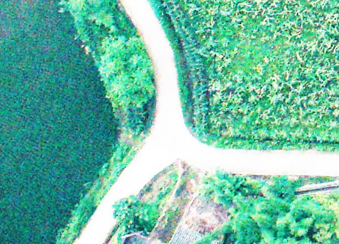
Due to the function of the square equilibrium, part of the gray level is submerged, the boundary line of the road at the three-way intersection has been lost, the whole road has completely turned white, and a lot of details have been lost. At present, there are many improvements of histogram equalization algorithm, one is based on HSI color space. Because the gray value of RGB color space is discrete integer value, it is easy to lose precision in the calculation process. The image is transformed from RGB color space to HSI color space, and the separated luminance I value is continuous transformation value, which is easier to retain more details in the process of square equalization. The first step is to convert RGB to HSI.

RGB to HSI Code:

public Double[] rgb2HSI(int[] rgb) {
		double sum = rgb[0] + rgb[1] + rgb[2];
		double r = rgb[0] / sum;
		double g = rgb[1] / sum;
		double b = rgb[2] / sum;
		double s1 = 0.5 * ((r - g) + (r - b));
		double s2 = Math.pow((r - g), 2) + (r - b) * (g - b);
		double s3 = s1 / Math.sqrt(s2);
		double h = 0.0;
		if (b <= g) {
			h = Math.acos(s3);
		} else if (b > g) {
			h = 2 * Math.PI - Math.acos(s3);
		}
		double s = 1 - 3 * Math.min(r, Math.min(g, b));
		double H = ((h * 180.0) / Math.PI);
		double S = s * 100.0;
		double I = sum / 3;
		return new Double[] { H, S, I };
	}

HSI conversion RGB Code:

public Integer[] hsi2RGB(Double[] hsi) {
		double h = (hsi[0] * Math.PI) / 180.0;
		double s = hsi[1] / 100.0;
		double i = hsi[2] / 255.0;
		double x = i * (1 - s);
		double y = i * (1 + (s * Math.cos(h)) / Math.cos(Math.PI / 3.0 - h));
		double z = 3 * i - (x + y);
		double r = 0, g = 0, b = 0;
		if (h < ((2 * Math.PI) / 3)) {
			b = x;
			r = y;
			g = z;
		} else if (h >= ((2 * Math.PI) / 3) && h < ((4 * Math.PI) / 3)) {
			h = h - ((2 * Math.PI) / 3.0);
			x = i * (1 - s);
			y = i * (1 + (s * Math.cos(h)) / Math.cos(Math.PI / 3.0 - h));
			z = 3 * i - (x + y);
			r = x;
			g = y;
			b = z;
		} else if (h >= ((4 * Math.PI) / 3) && h < ((2 * Math.PI))) {
			h = h - ((4 * Math.PI) / 3.0);
			x = i * (1 - s);
			y = i * (1 + (s * Math.cos(h)) / Math.cos(Math.PI / 3.0 - h));
			z = 3 * i - (x + y);
			g = x;
			b = y;
			r = z;
		}
		int red = (int) Math.round((r * 255));
		int green = (int) Math.round((g * 255));
		int blue = (int) Math.round((b * 255));
		return new Integer[] { red, green, blue};
	}

       

Although HSI color space can solve the problem of gray level loss in direct square equalization, the conversion between HSI and RGB color space needs a lot of calculation, resulting in slow image processing. Here is a solution for bloggers themselves.

Although it is easy to lose part of the gray level by using the traditional direct equalization, it can still use the traditional method to calculate the direct equalization. After the calculation of the direct equalization, the image and the original image can be fused for the mean value, and then the part of the lost gray value can be recovered. Although this method can not completely recover the lost gray level, it has been greatly improved compared with the traditional direct equalization. The processing flow is as follows: the original image is directly balanced and automatically colored, and the calculated image is fused to get the final image.

Design sketch:

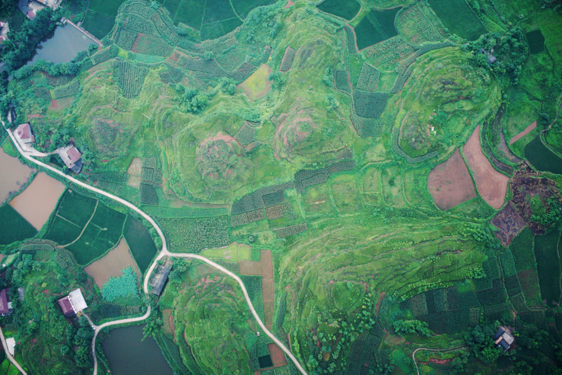
Compared with traditional square equalization, the image is darker after calculation, but more details can be retained. Let's look at the details.

From the enlarged details, the boundary line at the three-way intersection is still clear. The road is not completely white. 1.