Reference: https://blog.csdn.net/u013733326/article/details/79639509

After entering the post-graduate stage, the first thing I realized was the need to familiarize with and learn the neural network as soon as possible. I participated in a series of courses published by Teacher Wu Enda in NetEasy Cloud class, followed the course to complete the homework, and made a simple understanding and record.It is important to note that this paper is a simple summary and understanding based on the reference text. If you need to refer to the specific analysis of the algorithm, you can see the article referred to in this paper.

The next week's programming task is to complete a simple neural network that can recognize cats [the application of logistic regression]. As an introduction to the neural network, it can even be considered that the hidden layer is not involved, but the output is a 0/1 prediction of cats based on the input characteristics.

(1) Processing of input data

First, for each test sample, i.e., the image data currently input, based on the return value of lr_util.py, you can determine that it is the RGB information for the image and that the image size is.Taking train_set_x_orig as an example, assuming the number of training sets to be obtained is m, the dimension is.According to Teacher Wu's course, it is known that in order to keep the calculation speed as fast as possible, two vectorizations are usually needed: one of the input element layers of a test or training sample, and the other of all the sample layers (see Lessons 2.11-2.14):

1) First complete the vectorization of the first level:Array Reconstructed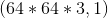Array;

2) Then complete the vectorization of the second level:From the vectorization of the first level, compress to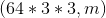Array;

The above steps complete the following steps mentioned in Teacher Wu Enda's coursereachThe vectorization process of.

    train_set_x_orig, train_set_y, test_set_x_orig, test_set_y, classes=load_dataset()


    m_train = train_set_y.shape[1]
    m_test = test_set_y.shape[1]
    num_px = train_set_x_orig.shape[1]

    train_set_x_flatten = train_set_x_orig.reshape(train_set_x_orig.shape[0],-1).T
    test_set_x_flatten = test_set_x_orig.reshape(test_set_x_orig.shape[0],-1).T
    train_set_x = train_set_x_flatten / 255
    test_set_x = test_set_x_flatten / 255

(2) Construction of neural networks

First, construct a Logistic regression function with the simplest formulaFor this prediction formula, firstInitialize to determine an initial value, then adjust the parameters gradually by gradient descent based on the training values.To achieve ultimately relatively reasonableValue of.In this process, there are two main steps:

1) Formula construction andInitialization

def initialize_with_zeros(dim):
    w = np.zeros(shape = (dim, 1))
    b = 0
    assert(w.shape == (dim, 1))
    assert(isinstance(b, float) or isinstance(b, int))
    return(w, b)

def sigmoind(z):
    s = 1/(1+np.exp(-z))
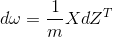
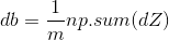
    return s

2) Gradient descent method: Teacher Wu Enda has 2.4 courseware for details of this process, the main formula involved is

                                                                          

                                                                          

                                                                         

                                                                          

                                                                         

# Cost and Gradient
def propagate(w,b,X,Y):
    m = X.shape[1]
    A = sigmoind(np.dot(w.T, X) + b)
    cost = (-1/m) * np.sum(Y * np.log(A) + (1-Y) * (np.log(1 - A)))

    dw = (1/m)*np.dot(X,(A-Y).T)
    db = (1/m)*np.sum(A-Y)

    assert(dw.shape == w.shape)
    assert(db.dtype == float)
    cost = np.squeeze(cost)
    assert(cost.shape == ())

    grads = {
        "dw":dw,
        "db":db
    }
    return(grads,cost)

# Run the gradient descent algorithm to optimize w and b
def optimize(w,b,X,Y,num_iterations,learning_rate,print_cost=False):
    costs = []
    for i in range(num_iterations):
        grads,cost = propagate(w,b,X,Y)
        dw = grads["dw"]
        db = grads["db"]

        w = w - learning_rate * dw
        b = b - learning_rate * db

        if i%100 == 0:
            costs.append(cost)
        if(print_cost) and (i % 100 == 0):
            print("Number of iterations: %i ， Error value: %f" % (i, cost))

        params = {
            "w" : w,
            "b" : b
        }
        grads = {
            "dw" : dw,
            "db" : db
        }
    return(params,grads,costs)

3) Calculating error: This process mainly involves the following formulas:

                                           

(3) Use of neural networks

Using the constructed neural network, the test set is tested, and the recognition error of each picture is obtained.

    

# Predicting labels using logistic functions
def predict(w,b,X):
    m = X.shape[1]
    Y_prediction = np.zeros((1,m))
    w = w.reshape(X.shape[0],1)

    A = sigmoind(np.dot(w.T, X) + b)
    for i in range(A.shape[1]):
        Y_prediction[0,i] = 1 if A[0,i] > 0.5 else 0
    assert(Y_prediction.shape == (1,m))

    return Y_prediction