Camera calibration often uses calibration boards. The common calibration methods are teacher Zhang Zhengyou's plate calibration. The common calibration boards are chessboard calibration board and disc calibration board. But in many places, when using TSAI two-step calibration method, do we use self-made calibration targets, such as our regular ordered cross targets, to get the following objects:

Method 1: Hough Line Detection to Find Intersection Points
In order to get the coordinates of the cross centers, the common method is to use hough line detection to get the expressions of all the vertical lines and get the coordinates of the intersection points by solving the intersection points, which I did, but in fact, we need to try many times to get the appropriate threshold and other parameters, that is to say, the generalization of the program is poor, which should also be written by my code. Not good, but really can not find a good method, because the selection of threshold parameters is indeed to be adjusted, and the same calibration board will be different between the light and shade, later I also want to avoid the acquisition of the latter points, only selected the first part of the cross with higher recognition, but because it is as the input of the calibration, so many points are enough. Of course, you can also fine-tune the parameters to get all the intersection points, but I have a cross in this calibration board because I made a mistake, so I filter out this line artificially.
front = imread('a.bmp');
back = imread('a_back.bmp');
%img = imread('cali.bmp');
img = front - back;
img_gray = rgb2gray(img);
%% Get row
thresh = graythresh(img_gray);
B = im2bw(img_gray, thresh);
B = bwmorph(B, 'skel', 1); % Skeleton extraction
B = bwmorph(B, 'spur', 2); % Deburring
[H, theta, rho] = hough(B, 'Theta', 30:0.03:89);
peaks = houghpeaks(H, 14);
rows = houghlines(B, theta, rho, peaks);
imshow(B), hold on;
temp = [];
row_line = [];
for k = 1:length(rows)
temp = [temp; rows(k).point1];
end
[temp, I] = sort(temp, 1, 'ASCEND');
for k = 1 : 6 % Number of rows expected
xy = [rows(I(k, 2)).point1, rows(I(k, 2)).point2];
plot([xy(1,1), xy(1, 3)], [xy(1,2), xy(1,4)], 'LineWidth', 2, 'Color', 'green');%Draw line segments
plot(xy(1,1), xy(1,2), 'x', 'LineWidth', 2, 'Color', 'yellow');%Starting point
plot(xy(1,3), xy(1,4), 'x', 'LineWidth', 2, 'Color', 'red');%End
row_line = [row_line; xy]; %[startX startY endX endY]
end
%% Get column
thresh = graythresh(img_gray);
B = im2bw(img_gray, thresh);
%B = bwmorph(B, 'skel', 1); % Skeleton extraction
%B = bwmorph(B, 'spur', 1); % Deburring
[H, theta, rho] = hough(B, 'Theta',-30:0.03:30);
peaks = houghpeaks(H, 7);
columns = houghlines(B, theta, rho, peaks);
%imshow(B),
hold on;
temp = [];
column_line = [];
for k = 1:length(columns)
temp = [temp; columns(k).point1];
end
[temp, I] = sort(temp, 1, 'ASCEND');
for k = 1 : 4 % Number of desired columns
xy = [columns(I(k, 1)).point1, columns(I(k, 1)).point2];
plot([xy(1,1), xy(1, 3)],[xy(1,2), xy(1,4)],'LineWidth',2,'Color','green');%Draw line segments
plot(xy(1,1),xy(1,2),'x','LineWidth',2,'Color','yellow');%Starting point
plot(xy(1,3),xy(1,4),'x','LineWidth',2,'Color','red');%End
column_line = [column_line; xy]; %[startX startY endX endY]
end
%% Obtaining intersection pixel coordinates
intersection = [];
line = [row_line; column_line];
for i = 1 : length(line) - 1
p1 = line(i, :);
k1 = (p1(2) - p1(4)) / (p1(1) - p1(3));
b1 = p1(2) - k1*p1(1);
for j = i+1 : length(line)
p2 = line(j, :);
k2 = (p2(2)-p2(4))/(p2(1)-p2(3));
b2 = p2(2)-k2*p2(1);
%Find the intersection point of two straight lines
x = -(b1-b2) / (k1-k2);
y = -(-b2*k1+b1*k2) / (k1-k2);
%Judging whether the intersection point may have a very similar slope on the two lines leads to a misunderstanding that the upper denominator is close to zero.
if min(p1(1),p1(3)) <= x && x <= max(p1(1),p1(3)) && ...
min(p1(2),p1(4)) <= y && y <= max(p1(2),p1(4)) && ...
min(p2(1),p2(3)) <= x && x <= max(p2(1),p2(3)) && ...
min(p2(2),p2(4)) <= y && y <= max(p2(2),p2(4))
plot(x,y,'.');
intersection = [intersection; [x, y]]; %First to last row and first to last row
end
end
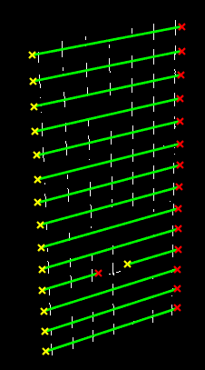
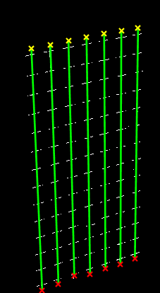
endThe results are as follows:
The intersection points of six rows and four rows have been calculated and marked in the four graphs (red dots).


Method 2: OpenCV Contour Finding and Template Matching
OpenCV is used to process the image. After simple processing, contour search is carried out to find all the cross contours, which may be mixed with the contours of noise points introduced by improper thresholds. But we can use contour area to restrict and find the appropriate size contours, which are actually the patterns of a cross target. We can use this as a template to search the object. The problem of multiple searches is that the contour obtained from a slightly left-right movement of a certain contour still has a high matching degree, so it will be recognized as a template, but it can not improve the recognition degree. Once the recognition degree requirement is improved, many targets that are not very clear will be lost. Therefore, when the recognition degree is slightly reduced (there must be a problem of repeated recognition), two contours will be compared. Relative distances are used to eliminate repetitive recognition objects, mainly by assigning all the similar targets to the first target (which may be a bit rough here, but also where errors occur). Then remove the same object and arrange all the points in the actual spatial order to correspond to the actual world coordinates (when calibration is needed). The code is as follows:
import numpy as np
import cv2
import os


GREEN = (0, 255, 0)
RED = (0,0,255)
filename = 'pixelCoordinate.txt'

# **** Basic processing of the original image and extract all contours ****
img = cv2.imread('cali.bmp')
imgray = cv2.cvtColor(img,cv2.COLOR_BGR2GRAY)
ret,thresh = cv2.threshold(imgray,30,255,0)
image, contours, hierarchy = cv2.findContours(thresh, cv2.RETR_TREE,cv2.CHAIN_APPROX_SIMPLE)

# ***********  Find an appropriate contour for the template   **********
for cnt in contours:
        if cv2.contourArea(cnt) > 120:
                (x,y,w,h) = cv2.boundingRect(cnt)
                template=imgray[y:y+h, x:x+w]
                rootdir=("C:/Users/Administrator/Desktop/cali/")
                if not os.path.isdir(rootdir):
                        os.makedirs(rootdir)
                cv2.imwrite( rootdir + "template.bmp",template)
                break

# ************ Find all matched contours ************
w, h = template.shape[::-1]
res = cv2.matchTemplate(imgray, template, cv2.TM_CCOEFF_NORMED)
threshold = 0.75

point = []
point_temp = []
loc = np.where(res >= threshold)
for pt in zip(*loc[::-1]):
        point.append([pt[0], pt[1]])
length = len(point)
print(' Before Processing:    ' + str(length))

# **** Assign the corresponding point of a similar template to one of them ******
i = 0
while(i < length):
        for j in range(i + 1, length):
                if ( np.abs(point[j][0] - point[i][0]) < 4 and np.abs(point[j][1] - point[i][1]) < 4):
                        point[j] = point[i]
        i = i + 1

# ***************** Eliminate similarities  *******************
for i in point:
        if i not in point_temp:
                point_temp.append(i)
print(' After Processing:    ' + str(len(point_temp)))


# ********** In order from left to right, from top to bottom ***********
point_temp.sort(key = lambda x:x[0])
for i in range(0, 92, 14):
        point_temp[i : i+14].sort(key = lambda x:x[1])


# ***************** Display and save the results **********************
if os.path.exists(filename):
        os.remove(filename)
for index in range(len(point_temp)):
        cv2.rectangle(img, tuple(point_temp[index]), (point_temp[index][0] + w, point_temp[index][1] + h), RED, 1)
        x = int(point_temp[index][0] + w/2)
        y = int(point_temp[index][1] + h/2)
        with open(filename, 'a') as file:
                file.write(str(x) + '  ' + str(y) + "\n")
                cv2.circle(img, (x, y), 0, GREEN, 0)

cv2.imshow('Result', img)
cv2.imwrite('Result.bmp', img)
The results are as follows:
