First, the main steps of a complete machine learning project process are given, as follows:
-
Project overview.
-
Get data.
-
Discover and visualize data and discover rules
-
Prepare data for machine learning algorithms.
-
Select models and train them.
-
Fine tuning model.
-
The solution is given.
-
Deployment, monitoring and maintenance system
1. Project overview
1.1 Delimitation Problem
When we start a machine learning project, we need to understand two questions first:
-
What are the business objectives? What do companies want to harvest from algorithms or models, which determines what algorithms and performance indicators need to be used?
-
How effective is the current solution?
Through these two problems, we can begin to design the system, that is, the solution.
But first of all, some questions need to be clarified:
-
Supervised or unsupervised, or intensive learning?
-
Is it classification, regression, or other types of problems?
-
Batch Learning or Online Learning
1.2 Selective Performance Indicators
Selective performance indicators usually refer to the accuracy of the model. In machine learning, the accuracy of the algorithm needs to be improved by reducing the loss, which requires the selection of an appropriate loss function to train the model.
Generally, the loss function can be divided into two categories from the type of learning task: regression loss and classification loss, which correspond to the regression problem and classification problem respectively.
Regression loss
Mean Square Error/Square Error/L2 Error
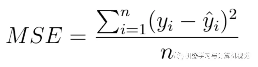
Mean Square Error (MSE) measures the mean square of the difference between the predicted value and the real value. It only considers the average size of the error, not its direction. But after squaring, the predicted values which deviate from the real values will be punished more severely, and the mathematical characteristics of MSE are very good, that is, it is particularly easy to derive, so it will be easier to calculate the gradient.
The mathematical formula of MSE is as follows:
The code is implemented as follows:
def rmse(predictions, targets):
    #Errors between real and predicted values
    differences = predictions - targets
    differences_squared = differences ** 2
    mean_of_differences_squared = differences_squared.mean()
    #Take the square root
    rmse_val = np.sqrt(mean_of_differences_squared)
    return rmse_val
Of course, the above code implements root mean square error (RMSE). A simple test example is as follows:
y_hat = np.array([0.000, 0.166, 0.333])
y_true = np.array([0.000, 0.254, 0.998])

print("d is: " + str(["%.8f" % elem for elem in y_hat]))
print("p is: " + str(["%.8f" % elem for elem in y_true]))
rmse_val = rmse(y_hat, y_true)
print("rms error is: " + str(rmse_val))
The output results are as follows:
d is: ['0.00000000', '0.16600000', '0.33300000']
p is: ['0.00000000', '0.25400000', '0.99800000']
rms error is: 0.387284994115
Square absolute error/L1 error
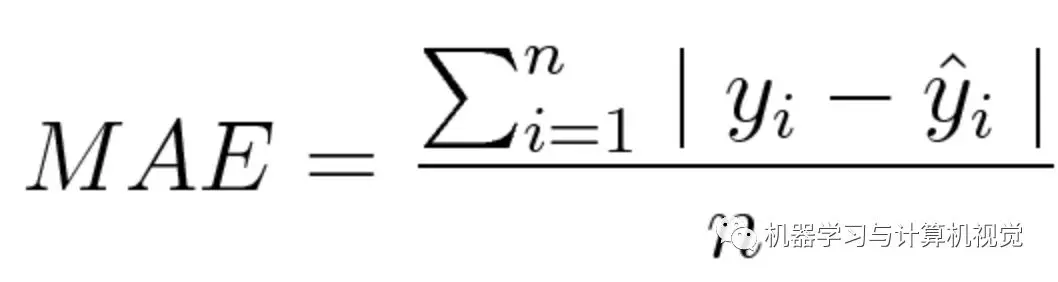
The mean absolute error (MAE) measures the average value of the sum of the absolute differences between the predicted and the observed values. Like MSE, this measurement method measures the error size without considering the direction. But the difference between MAE and MSE is that MAE needs more complex tools like linear programming to calculate gradients. In addition, MAE is more robust to outliers because it does not use squares.
The mathematical formulas are as follows:
The code implementation of MAE is not difficult, as follows:
def mae(predictions, targets):
    differences = predictions - targets
    absolute_differences = np.absolute(differences)
    mean_absolute_differences = absolute_differences.mean()
    return mean_absolute_differences
The test sample can directly use the MSE test code just now. The output results are as follows:
d is: ['0.00000000', '0.16600000', '0.33300000']
p is: ['0.00000000', '0.25400000', '0.99800000']
mae error is: 0.251
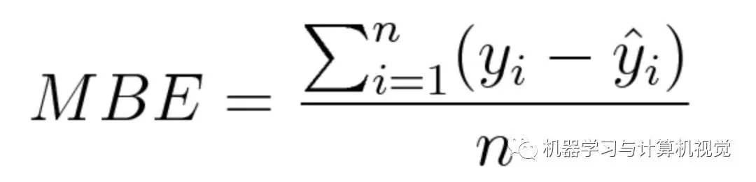
Mean bias error
This loss function is seldom used, and it is very uncommon in the field of machine learning. This is the first time I have seen this loss function. It's very similar to MAE, the only difference is that it doesn't use absolute values. Therefore, it should be noted that the positive and negative errors can offset each other. Although it is not so accurate in practical application, it can determine whether there are positive or negative deviations in the model.
The mathematical formulas are as follows:
Code implementation, in fact, only need to delete the code added absolute value on the basis of MAE, as follows:
def mbe(predictions, targets):
    differences = predictions - targets
    mean_absolute_differences = differences.mean()
    return mean_absolute_differences
The results are as follows:
d is: ['0.00000000', '0.16600000', '0.33300000']
p is: ['0.00000000', '0.25400000', '0.99800000']
mbe error is: -0.251
We can see that there is a negative deviation in the simple test sample we gave.
Classification error
Hinge Loss/Multi-Classification SVM Error
hinge loss is commonly used in maximum-margin classification, which is within a certain security interval (usually 1), and the correct category should score higher than the sum of all error categories. Support Vector Machine (SVM) is the most commonly used method. Although not differentiable, it is a convex function and can be used as a convex optimizer commonly used in machine learning.
Its mathematical formula is as follows:
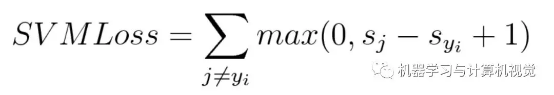
In the formula, sj denotes the predicted value, while s_yi is the true value, or the correct predicted value, while 1 denotes the margin. Here we hope that the similarity between the two predicted results can be expressed by the difference between the real value and the predicted value, while margin is a safety factor set artificially. We hope that the correct classification score is higher than the wrong prediction score, and higher than a margin value, that is, the higher the s_yi, the better the lower the s_j. The calculated Loss tends to zero.
To illustrate with a simple example, suppose there are three training samples as follows, we need to predict three categories. The values in the table below are the values of each category obtained by the algorithm:
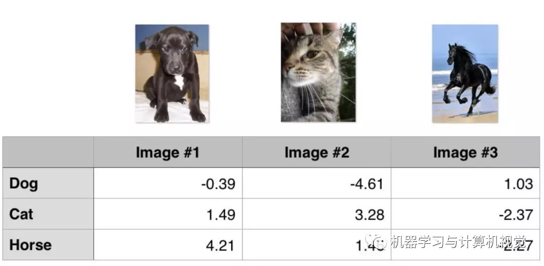
Each column is the number of each category in each picture. We can also know that the real values of each column are dogs, cats and horses. The simple code implementation is as follows:
def hinge_loss(predictions, label):
    '''
    hinge_loss = max(0, s_j - s_yi +1)
    :param predictions:
    :param label:
    :return:
    '''
    result = 0.0
    pred_value = predictions[label]
    for i, val in enumerate(predictions):
        if i == label:
            continue
        tmp = val - pred_value + 1
        result += max(0, tmp)
    return result
The test examples are as follows:
image1 = np.array([-0.39, 1.49, 4.21])
image2 = np.array([-4.61, 3.28, 1.46])
image3 = np.array([1.03, -2.37, -2.27])
result1 = hinge_loss(image1, 0)
result2 = hinge_loss(image2, 1)
result3 = hinge_loss(image3, 2)
print('image1,hinge loss={}'.format(result1))
print('image2,hinge loss={}'.format(result2))
print('image3,hinge loss={}'.format(result3))

#Output results
# image1,hinge loss=8.48
# image2,hinge loss=0.0
# image3,hinge loss=5.199999999999999
This calculation process is more vividly illustrated:
## 1st training example
max(0, (1.49) - (-0.39) + 1) + max(0, (4.21) - (-0.39) + 1)
max(0, 2.88) + max(0, 5.6)
2.88 + 5.6
8.48 (High loss as very wrong prediction)
## 2nd training example
max(0, (-4.61) - (3.28)+ 1) + max(0, (1.46) - (3.28)+ 1)
max(0, -6.89) + max(0, -0.82)
0 + 0
0 (Zero loss as correct prediction)
## 3rd training example
max(0, (1.03) - (-2.27)+ 1) + max(0, (-2.37) - (-2.27)+ 1)
max(0, 4.3) + max(0, 0.9)
4.3 + 0.9
5.2 (High loss as very wrong prediction)
By calculation, the higher the hinge loss value, the more inaccurate the prediction will be.
Cross Entropy Loss/Negative Logarithmic Likelihood
cross entroy loss is the most commonly used loss function in classification algorithm.
Mathematical formulas:

According to the formula, if the actual label y_i is 1, then the formula has only the first half; if it is 0, then only the second half. Simply put, cross-entropy multiplies the logarithm of the probability of predicting the true category, and it punishes those values with high confidence but incorrect prediction.
The code is implemented as follows:
def cross_entropy(predictions, targets, epsilon=1e-10):
    predictions = np.clip(predictions, epsilon, 1. - epsilon)
    N = predictions.shape[0]
    ce_loss = -np.sum(np.sum(targets * np.log(predictions + 1e-5))) / N
    return ce_loss
Examples of test samples are as follows:
predictions = np.array([[0.25, 0.25, 0.25, 0.25],
                            [0.01, 0.01, 0.01, 0.96]])
targets = np.array([[0, 0, 0, 1],
                    [0, 0, 0, 1]])
cross_entropy_loss = cross_entropy(predictions, targets)
print("Cross entropy loss is: " + str(cross_entropy_loss))

#Output results
# Cross entropy loss is: 0.713532969914
For the above code example, source code address:
https://github.com/ccc013/CodesNotes/blob/master/hands_on_ml_with_tf_and_sklearn/Loss_functions_practise.py