After learning the basic knowledge of data analysis, I hope to consolidate knowledge through practical exercises, introductory data contest, and share with you some introductory kernel s on kaggle to integrate the resources I use and the learning process.
Home Credit Default Risk
Address: https://www.kaggle.com/willkoehrsen/start-here-a-gentle-introduction
Author's homepage: https://www.kaggle.com/willkoehrsen
Background: Home Credit uses a variety of alternative data (including telecommunications and transaction information) to predict the repayment ability of its customers.
Data resources: https://pan.baidu.com/s/1uaMESw1ca_Y9O3YVfrSrEA
Extraction code: d13i
Content: Based on the original author's content, combined with my own understanding and learning of some knowledge points, I also write some reflections on my own practical operation, which is suitable for beginners to learn.
Previous links:
Kaggle_Kernel Learning_Home Credit Default Risk_EDA
In the last blog, we explored the most prominent positive and negative correlation variables, and also discussed some related work of Feature Engineering and machine learning according to their influencing factors.
Feature engineering is a basic process, which can include feature construction: adding new features from existing data, and feature selection: selecting only the most important features or other dimension reduction methods. We can use many techniques to create and select features. This paper mainly uses Polynomial Features and Domain knowledge features to construct and adjust features.
1. Polynomial Features Generation from Polynomial Features
In this method, the function we create is the existing strong correlation features and the interaction items between these features. For example, we can create variables EXT_SOURCE_1^ 2 and EXT_SOURCE_2^ 2, as well as variables such as EXT_SOURCE_1 x EXT_SOURCE_2, EXT_SOURCE_1 xEXT_SOURCE_2^2, EXT_SOURCE_1^ 2, EXT_SOURCE_2^2, EXT_SOURCE_1^ 2, EXT_SOURCE 2^2,
And so on. These functions, which are composed of multiple individual variables, are called interaction items because they capture interactions between variables. In other words, although the two variables themselves may not have a strong impact on the target, combining them to form an interactive variable may show the relationship with the target.
# Extracting Several Strongly Related Features and TARGET Attributes
poly_features_train = data_train[['EXT_SOURCE_1','EXT_SOURCE_2','EXT_SOURCE_3','DAYS_BIRTH','TARGET']]
poly_features_test = data_test[['EXT_SOURCE_1','EXT_SOURCE_2','EXT_SOURCE_3','DAYS_BIRTH']]
# Store TARGET separately
poly_target = poly_features_train['TARGET']
# Remove TARGET and keep test / train consistent
poly_features_train = poly_features_train.drop(columns=['TARGET'])
Imputer interpolation is used to fill in the gaps before the change.
from sklearn.preprocessing import Imputer
# The strategy is to fill in the middle value
impt = Imputer(strategy='median')
# Transform directly with fit_transform method
# Note that the result is a digital matrix.
poly_features_train = impt.fit_transform(poly_features_train)
poly_features_test = impt.fit_transform(poly_features_test)
poly_features_train
array([[8.30369674e-02, 2.62948593e-01, 1.39375780e-01, 9.46100000e+03],
       [3.11267311e-01, 6.22245775e-01, 5.35276250e-01, 1.67650000e+04],
       [5.05997931e-01, 5.55912083e-01, 7.29566691e-01, 1.90460000e+04],
       ...,
       [7.44026400e-01, 5.35721752e-01, 2.18859082e-01, 1.49660000e+04],
       [5.05997931e-01, 5.14162820e-01, 6.61023539e-01, 1.19610000e+04],
       [7.34459669e-01, 7.08568896e-01, 1.13922396e-01, 1.68560000e+04]])
Call Polynomial Features for transformation
from sklearn.preprocessing import PolynomialFeatures
poly_transformer = PolynomialFeatures(degree=3)
poly_transformer.fit(poly_features_train)
poly_features_train = poly_transformer.transform(poly_features_train)
poly_features_test = poly_transformer.transform(poly_features_test)
The original columns need to be renamed due to the loss of them
# Invoke the get_feature_names() method to see the polynomial composition generated by the input variable when degree = 3
# Note that the order used to construct the DataFrame is the same
poly_transformer.get_feature_names(input_features=['EXT_SOURCE_1', 'EXT_SOURCE_2', 'EXT_SOURCE_3', 'DAYS_BIRTH'])[:15]
['1',
 'EXT_SOURCE_1',
 'EXT_SOURCE_2',
 'EXT_SOURCE_3',
 'DAYS_BIRTH',
 'EXT_SOURCE_1^2',
 'EXT_SOURCE_1 EXT_SOURCE_2',
 'EXT_SOURCE_1 EXT_SOURCE_3',
 'EXT_SOURCE_1 DAYS_BIRTH',
 'EXT_SOURCE_2^2',
 'EXT_SOURCE_2 EXT_SOURCE_3',
 'EXT_SOURCE_2 DAYS_BIRTH',
 'EXT_SOURCE_3^2',
 'EXT_SOURCE_3 DAYS_BIRTH',
 'DAYS_BIRTH^2',
 'EXT_SOURCE_1^3',
 'EXT_SOURCE_1^2 EXT_SOURCE_2',
 'EXT_SOURCE_1^2 EXT_SOURCE_3',
 'EXT_SOURCE_1^2 DAYS_BIRTH',
 'EXT_SOURCE_1 EXT_SOURCE_2^2',
 'EXT_SOURCE_1 EXT_SOURCE_2 EXT_SOURCE_3',
 'EXT_SOURCE_1 EXT_SOURCE_2 DAYS_BIRTH',
 'EXT_SOURCE_1 EXT_SOURCE_3^2',
 'EXT_SOURCE_1 EXT_SOURCE_3 DAYS_BIRTH',
 'EXT_SOURCE_1 DAYS_BIRTH^2',
 'EXT_SOURCE_2^3',
 'EXT_SOURCE_2^2 EXT_SOURCE_3',
 'EXT_SOURCE_2^2 DAYS_BIRTH',
 'EXT_SOURCE_2 EXT_SOURCE_3^2',
 'EXT_SOURCE_2 EXT_SOURCE_3 DAYS_BIRTH',
 'EXT_SOURCE_2 DAYS_BIRTH^2',
 'EXT_SOURCE_3^3',
 'EXT_SOURCE_3^2 DAYS_BIRTH',
 'EXT_SOURCE_3 DAYS_BIRTH^2',
 'DAYS_BIRTH^3']
# Converting existing column names and data to Dataframe
poly_features_train = pd.DataFrame(poly_features_train,
                                   columns=poly_transformer.get_feature_names([
                                       'EXT_SOURCE_1', 'EXT_SOURCE_2',
                                       'EXT_SOURCE_3', 'DAYS_BIRTH'
                                   ]))
poly_features_test = pd.DataFrame(poly_features_test,
                                 columns=poly_transformer.get_feature_names([
                                      'EXT_SOURCE_1', 'EXT_SOURCE_2',
                                       'EXT_SOURCE_3', 'DAYS_BIRTH'
                                 ]))
poly_features_train.head()
View new property dependencies
# Growth of objective function
poly_features['TARGET'] = poly_target
# Find the correlation coefficient
poly_corrs = poly_features.corr()['TARGET'].sort_values()
# View Extremum
print('head:\n',poly_corrs.head(5))
print('\ntail:\n',poly_corrs.tail(5))
head:
EXT_SOURCE_2 EXT_SOURCE_3                -0.193939
EXT_SOURCE_1 EXT_SOURCE_2 EXT_SOURCE_3   -0.189605
EXT_SOURCE_2 EXT_SOURCE_3 DAYS_BIRTH     -0.181283
EXT_SOURCE_2^2 EXT_SOURCE_3              -0.176428
EXT_SOURCE_2 EXT_SOURCE_3^2              -0.172282
Name: TARGET, dtype: float64

tail:
DAYS_BIRTH     -0.078239
DAYS_BIRTH^2   -0.076672
DAYS_BIRTH^3   -0.074273
TARGET          1.000000
1                    NaN
Name: TARGET, dtype: float64
Combining the new features with the original DataFrame
# Select SK_ID_CURR as the join column
poly_features_train['SK_ID_CURR'] = data_train['SK_ID_CURR']
poly_features_test['SK_ID_CURR'] = data_test['SK_ID_CURR']

# Parameter on to specify the primary key for data set merging
data_train_poly = data_train.merge(poly_features_train, on='SK_ID_CURR', how='left')
data_test_poly = data_test.merge(poly_features_test, on='SK_ID_CURR', how='left')
# Uniform column
data_train_poly, data_test_poly = data_train_poly.align(data_test_poly, join='inner',axis=1)
# View Dimensions
print('Dimension of training set after polynomial generation: ', data_train_poly.shape)
print('Test Set Dimensions after Polynomial Generation: ', data_test_poly.shape)
Dimensions of training set after polynomial generation: (307511, 275)
Dimensions of test set after polynomial generation: (48744, 275)
2. New features of domain knowledge construction
CREDIT_INCOME_PERCENT: Percentage of Credit to Customer Income
ANNUITY_INCOME_PERCENT: Percentage of loan annuity relative to customer income
CREDIT_TERM: Term of payment in monthly units (because annuity is the amount due each month)
DAYS_EMPLOYED_PERCENT: Number of days of employment relative to customer age
data_train_domain = data_train.copy()
data_test_domain = data_test.copy()

# Separate structural features

# Part Construction of Training Set
data_train_domain['CREDIT_INCOME_PERCENT'] = data_train_domain['AMT_CREDIT'] / data_train_domain['AMT_INCOME_TOTAL']
data_train_domain['ANNUITY_INCOME_PERCENT'] = data_train_domain['AMT_ANNUITY'] / data_train_domain['AMT_INCOME_TOTAL']
data_train_domain['CREDIT_TERM'] = data_train_domain['AMT_ANNUITY'] / data_train_domain['AMT_CREDIT']
data_train_domain['DAYS_EMPLOYED_PERCENT'] = data_train_domain['DAYS_EMPLOYED'] / data_train_domain['DAYS_BIRTH']

# Part Construction of Test Set
data_test_domain['CREDIT_INCOME_PERCENT'] = data_test_domain['AMT_CREDIT'] / data_test_domain['AMT_INCOME_TOTAL']
data_test_domain['ANNUITY_INCOME_PERCENT'] = data_test_domain['AMT_ANNUITY'] / data_test_domain['AMT_INCOME_TOTAL']
data_test_domain['CREDIT_TERM'] = data_test_domain['AMT_ANNUITY'] / data_test_domain['AMT_CREDIT']
data_test_domain['DAYS_EMPLOYED_PERCENT'] = data_test_domain['DAYS_EMPLOYED'] / data_test_domain['DAYS_BIRTH']
plt.figure(figsize = (8, 16))
# iteration
for i, feature in enumerate(['CREDIT_INCOME_PERCENT', 'ANNUITY_INCOME_PERCENT', 'CREDIT_TERM', 'DAYS_EMPLOYED_PERCENT']):
    # subplot drawing subgraph
    plt.subplot(4, 1, i + 1)

    # repay
    sns.kdeplot(data_train_domain.loc[data_train_domain['TARGET'] == 0, feature], label = 'target == 0')
    # Be overdue
    sns.kdeplot(data_train_domain.loc[data_train_domain['TARGET'] == 1, feature], label = 'target == 1')

    # Label
    plt.title('Distribution of %s by Target Value' % feature)
    plt.xlabel('%s' % feature);
    plt.ylabel('Density');

plt.tight_layout(h_pad = 2.5)
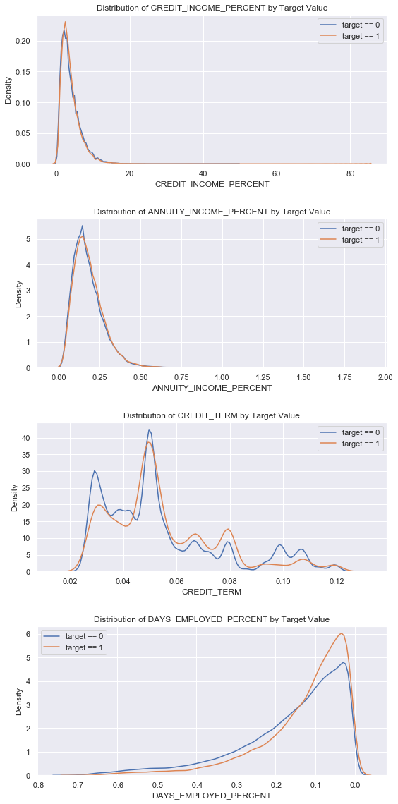
data_corr = data_train_domain[['CREDIT_INCOME_PERCENT', 'ANNUITY_INCOME_PERCENT', 'CREDIT_TERM', 'DAYS_EMPLOYED_PERCENT','TARGET']]
data_corr.corr()['TARGET']
CREDIT_INCOME_PERCENT    -0.007727
ANNUITY_INCOME_PERCENT    0.014265
CREDIT_TERM               0.012704
DAYS_EMPLOYED_PERCENT     0.067955
TARGET                    1.000000
Name: TARGET, dtype: float64
Looking at the correlation coefficient, it's hard to say whether it works or not.
BASELINE
Some of the previous processing is just to explore the possibility of data, not complete data preprocessing, here still need to go a set of first.
preprocessing process
# Import related modules including normalization/interpolation
from sklearn.preprocessing import MinMaxScaler, Imputer

# Separation of TARGET
if 'TARGET' in data_train:
    train = data_train.drop(columns = ['TARGET'])
else:
    train = data_train.copy()

# Test Set
test = data_test.copy()
# Median Filling
imputer = Imputer(strategy = 'median')

# Data range conversion to 0-1
scaler = MinMaxScaler(feature_range = (0, 1))

# train
imputer.fit(train)
scaler.fit(train)
# Imputer transformation
train = imputer.transform(train)
test = imputer.transform(test)

# MinMax Scaler transformation
train = scaler.transform(train)
test = scaler.transform(test)
print('Training data shape: ', train.shape)
print('Testing data shape: ', test.shape)
Training data shape:  (307511, 240)
Testing data shape:  (48744, 240)
Make a baseline prediction
from sklearn.linear_model import LogisticRegression

# No search
log_reg = LogisticRegression(C = 0.0001)

#train
log_reg.fit(train, train_labels)
LogisticRegression(C=0.0001, class_weight=None, dual=False,
          fit_intercept=True, intercept_scaling=1, max_iter=100,
          multi_class='warn', n_jobs=None, penalty='l2', random_state=None,
          solver='warn', tol=0.0001, verbose=0, warm_start=False)
# Using Predict_proba() Method to Predict the Possibility of Result 1
# Converted to a prediction of the probability of eventual overdue
log_reg_pred = log_reg.predict_proba(test)[:, 1]
# Construct Dataframe to prepare for submission
submit = data_test[['SK_ID_CURR']]
submit['TARGET'] = log_reg_pred
submit.head()
	SK_ID_CURR	TARGET
0	100001		0.087750
1	100005		0.163957
2	100013		0.110238
3	100028		0.076575
4	100038		0.154924
# Save as csv
submit.to_csv('log_reg_baseline.csv', index = False)