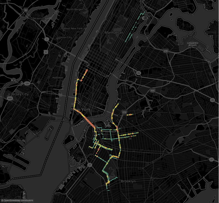
Measuring the quality of NYC Bike Lanes through street imagery

• stay Another article In this article, I will briefly introduce the image processing and computer vision technologies we use for street images.
  We've also tried to use it Microsoft Custom Visual Products, based on the simple marking of bicycle lane images, quickly generate classification results.

• python has a powerful image processing capability, which makes it popular openCV and SciPy Library.

• Greg Dobler The professor is an image processing expert at NYU CUSP and we consulted him to help us build these algorithms.

• We try to evaluate the quality of bicycle paths in four ways, and learn from them NACTO's Guide to Urban Street Design:

  1. The riding quality is measured using the acceleration data recorded by the app mentioned earlier.
  2. The color of bicycle lanes, green lanes are better than untouched ones because they have better visibility.
  3. Symbols and road markings, good markings for better road quality.
  4. Visible road defects, such as cracks and pits, are as small as possible.

• The following emphasis is on Measuring Pavement Markers and visible defects.This is a naive scoring system and the first iteration of the program (similar to many computer vision applications).

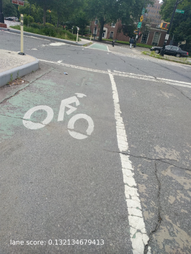
Detecting lane markers

• Use SciPy to read the original image and display it

import scipy.ndimage as nd
photoName = 'path'
img = nd.imread(photoName)

import matplotlib.pylab as plt
def plti(im, **kwargs):
    """
    //Auxiliary Functions for Drawing
    """
    plt.imshow(im, interpolation="none", **kwargs)
    plt.axis('off') # Remove axes
    plt.show() # Pop-up window display image
plti(img)

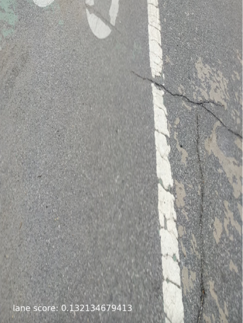
• Cut out the top half of the picture (removing features of non-bicycle lanes) and the bottom 10% (removing my bicycle tires) (this feature is not shown in the above image)

#Number of rows and columns in the picture
nrow, ncol = img.shape[:2]
#Starting at half the number of rows until 0.9 rows
img = img[nrow//2:(nrow-nrow//10),:,:]

plti(img)

• Use color thresholds to filter the clipped image and generate a binary graph (black and white)

#Separate three layers of color
red, grn, blu = img.transpose(2, 0, 1)
#Applying threshold processing
thrs = 200
wind = (red > thrs) & (grn > thrs) & (blu > thrs)

plti(wind)

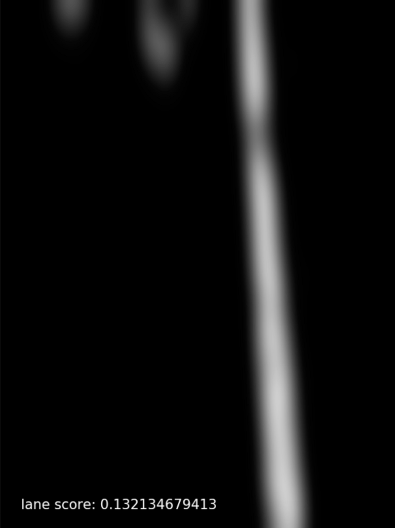
• Next, use Gaussian blur with a bandwidth value of 40 pixels

# Fuzzy White Blocks Using Gauss Filtering
gf = nd.filters.gaussian_filter
blurPhoto = gf(1.0 * wind, 40)

plti(blurPhoto)

• Set threshold again, 0,1 binary image

# Gray area with threshold between black and white
# Pixel value greater than threshold 1, less than 0
threshold = 0.16
wreg = blurPhoto > threshold

plti(wreg)

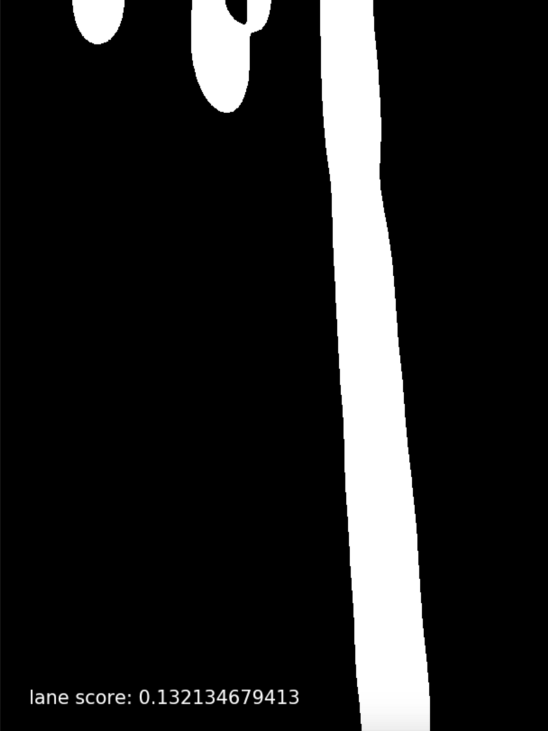
The final score for the lane marker is: the percentage of white areas (i.e., Lane markers) in the last image (wreg.mean()).This is 13.2%.

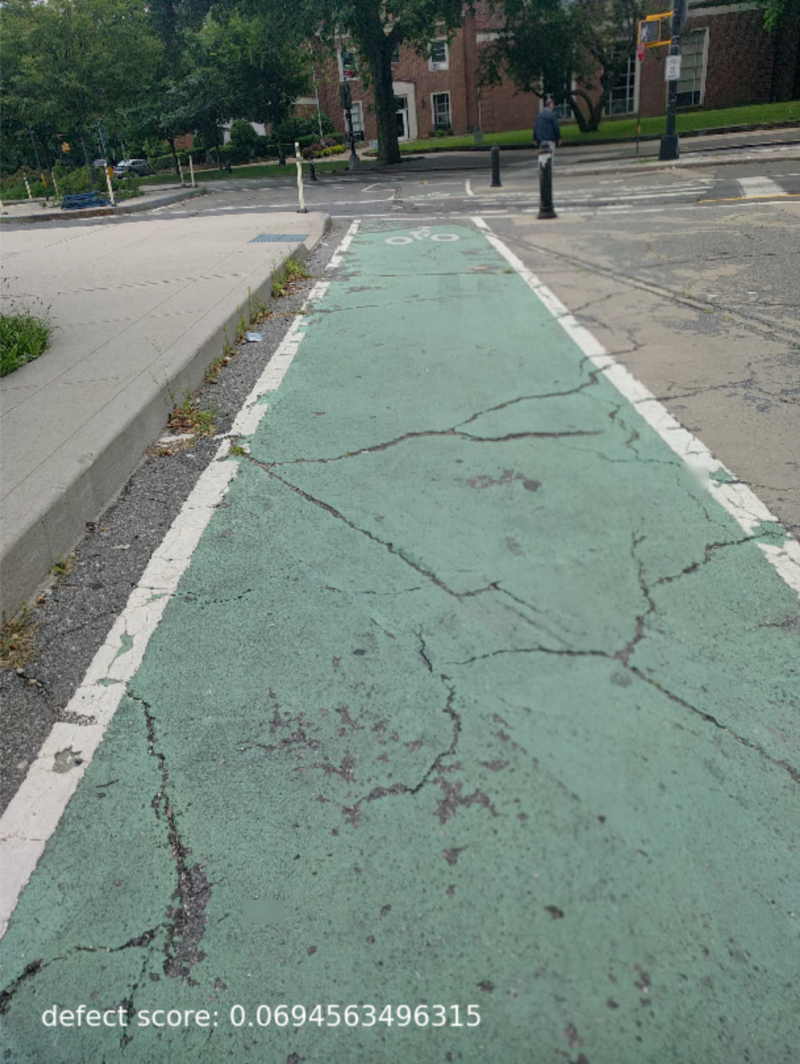
Detecting visible road defects

• Read pictures

import scipy.ndimage as nd
photoName = r'path'
img = nd.imread(photoName)

plti(img)

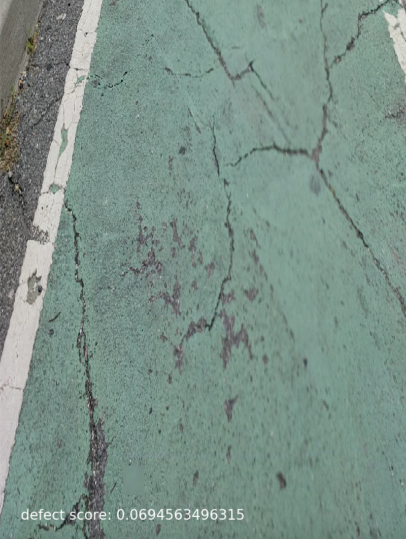
• Same clipping as above

#Number of rows and columns in the picture
nrow, ncol = img.shape[:2]
#Starting at half the number of rows until 0.9 rows
img = img[nrow//2:(nrow-nrow//10),:,:]

plti(img)

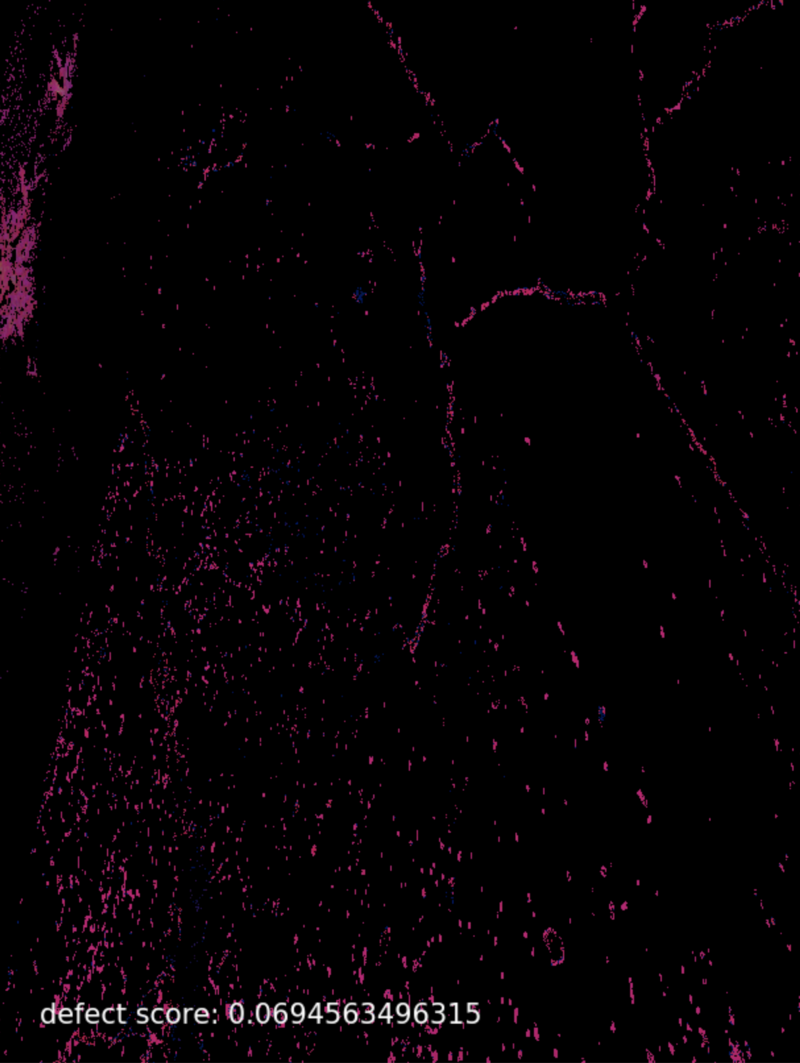
• Filter, use here median filtering To preserve edges

md = nd.filters.median_filter
# blurred image
md_blurPhoto = md(img, 5)
plti(md_blurPhoto)

• From image RGB Convert to HSV And filter the image to keep only the darker (defective) pixels

import cv2
lower = np.array([0, 10, 50])
upper = np.array([360, 100, 100])
hls = cv2.cvtColor(md_blurPhoto, cv2.COLOR_BGR2HSV)
mask = cv2.inRange(hls, lower, upper)
res = cv2.bitwise_and(hls, hls, mask = mask)

• Edge detection, using canny edge detection.
  We also applied a 3x3 Gaussian filter to the image, then eroded/expanded the remaining white pixels to eliminate noise.

edges_cv = cv2.Canny(res, 200, 400)
#Blur Edge
blurred_edges = cv2.GaussianBlur(edges_cv,(3,3),0) 
# Only want to preserve cracks that are adjacent to other cracks or larger than a minimum threshold
bdilation = nd.morphology.binary_dilation
berosion = nd.morphology.binary_erosion
edges_2 = bdilation(berosion(blurred_edges, iterations=2), iterations=2)
defect_score = edges_2.mean()

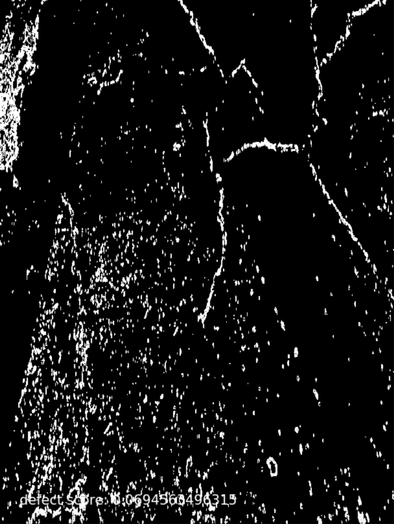
• The final defect score is 6.95%, which is the percentage of white pixels in the image processed above.

• Again, these techniques are only the first iteration and are limited by changes in light or camera angles.However, they are sufficient to measure the quality of some of the bike lanes we have seen so far in New York City.

So far, the team has ridden more than 50 miles and collected 4500 street views

• Further, a convolution neural network (CNN) can be constructed and trained with each of our (tagged) images.