problem

solution

As a little white, I really did not find any suitable way, so I can only consult the papers of the big guys, found a very good one, and retailed it.
The original link is as follows
http://www.yndxxb.ynu.edu.cn/yndxxb/article/2018/0258-7971-40-5-879.html#outline_anchor_7

1 Data analysis

1.1 Data Visualization

This part is not very difficult, that is, reading data and drawing.

1.1.1 Read all data and draw pictures

To read all the data, just open excel and take out the contents of the corresponding fields. We need to pay attention to the processing of time type.

data = xlrd.open_workbook("2018 Northeast Three Provinces Mathematical Modeling League F Annex.xls")  # Open excel
    table = data.sheet_by_name("Lambert 20140 415-0612")  # Read sheet
    times = []
    flow1 = []
    flow2 = []
    for i in range(1, table.nrows):
        row = table.row_values(i)  # Line data in an array
        date = xldate_as_tuple(row[0], 0)		# Date tuple
        times.append(datetime.datetime(*date))
        flow1.append(row[1])
        flow2.append(row[2])
    draw_all(times, flow1, flow2)

Drawing directly from the read data still requires attention to the processing of time types.

def draw_all(times, flow1, flow2):
    # Configure abscissa
    length = len(times)
    coordinate = [times[0], times[int(length / 4)], times[int(2 * length / 4)], times[int(3 * length / 4)],
                  times[length - 1]]
    plt.xticks(coordinate)
    plt.gca().xaxis.set_major_formatter(mdates.DateFormatter('%m-%d'))
    # Configure title, axis name
    plt.title("ALL DAY")
    plt.xlabel("time")
    plt.ylabel("flow (L/s)")
    # Plot
    plt.plot(times, flow1, label='DMA1')
    plt.plot(times, flow2, label='DMA2')
    plt.legend(loc=4)  # Specify the location of legend so that readers can help themselves with its usage
    plt.gcf().autofmt_xdate()  # Automatic Rotation Date Marker
    plt.show()

give the result as follows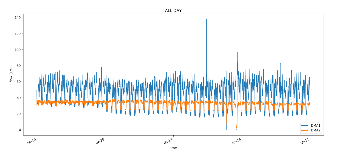

1.1.2 Read the data of a certain day and draw a picture

Notice here how to determine the date of reading the data as specified.

def read_oneday(month, day):
    '''
    :param month: Designated month
    :param day: Designated days
    :return:    There is no return value, but the drawing method is then invoked. May also times,flow Return to the main function call
    '''
    data = xlrd.open_workbook("2018 Northeast Three Provinces Mathematical Modeling League in 1997 F Annex.xls")  # Open excel
    table = data.sheet_by_name("Lambert 20140 415-0612")  # Read sheet
    times = []
    flow1 = []
    flow2 = []
    for i in range(1, table.nrows):
        row = table.row_values(i)  # Line data in an array
        date = xldate_as_tuple(row[0], 0)
        if date[1] == month and date[2] == day:
            times.append(datetime.datetime(*date))
            flow1.append(row[1])
            flow2.append(row[2])
    draw_oneday(times, flow1, flow2)

Compared with the previous drawing, the coordinate axes and headings need to be modified, and attention should still be paid to date processing.

def draw_oneday(times, flow1, flow2):
    # Configuration abscissa
    length = len(times)
    coordinate = [times[0], times[int(length / 4)], times[int(2 * length / 4)], times[int(3 * length / 4)],
                  times[length - 1]]
    plt.xticks(coordinate)
    plt.gca().xaxis.set_major_formatter(mdates.DateFormatter('%H:%M:%S'))
    # Configure title, axis name
    plt.title(times[0].strftime('%Y/%m/%d'))
    plt.xlabel("time")
    plt.ylabel("flow (L/s)")
    # Plot
    plt.plot(times, flow1, label='DMA1')
    plt.plot(times, flow2,  label='DMA2')
    plt.legend(loc=4)  # Specify the location of legend so that readers can help themselves with its usage
    plt.gcf().autofmt_xdate()  # Automatic Rotation Date Marker
    plt.show()

give the result as follows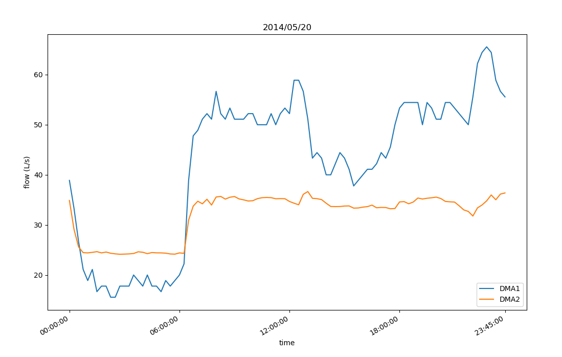

1.2 Water Flow

Find out the daily water leakage first.

def find_leak():
    data = xlrd.open_workbook("2018 Northeast Three Provinces Mathematical Modeling League in 1997 F Annex.xls")  # Open excel
    table = data.sheet_by_name("Lambert 20140 415-0612")  # Read sheet
    # Leakage, dictionary type, key date, value for the day of leakage
    leak1 = {}
    leak2 = {}
    # Minimum flow at 2-5 points of the day as leakage
    minFlow1 = 999
    minFlow2 = 999
    for i in range(1, table.nrows):
        row = table.row_values(i)  # Line data in an array
        date = xldate_as_tuple(row[0], 0)
        if i != 1 and date[2] != oldDate[2]:  # Compare date changes
            key = str(oldDate[1])+"-"+str(oldDate[2])
            leak1[key] = minFlow1
            leak2[key] = minFlow2
            minFlow1 = 999
            minFlow2 = 999
        if date[3] >= 2 and date[3] <= 5:
            minFlow1 = min(minFlow1, row[1])
            minFlow2 = min(minFlow2, row[2])
        oldDate = date  # Record a date
        if i == table.nrows - 1:                        ##Deal with the last day alone
            key = str(date[1]) + "-" + str(date[2])
            leak1[key] = minFlow1
            leak2[key] = minFlow2
    return leak1, leak2

Calculate water consumption according to water leakage, pay attention to replacing negative number with 0.

def cal_usewater():
    data = xlrd.open_workbook("result.xls")  # Open excel
    table = data.sheet_by_name("Lambert 20140 415-0612")  # Read sheet
    from xlutils.copy import copy
    wb = xlutils.copy.copy(data)
    sheet = wb.get_sheet(0)
    sheet.write(0, 3, 'use1')
    sheet.write(0, 4, 'use2')
    leak1, leak2 = find_leak()
    for i in range(1, table.nrows):
        row = table.row_values(i)  # Line data in an array
        date = xldate_as_tuple(row[0], 0)
        key = str(date[1]) + "-" + str(date[2])
        sheet.write(i, 3, str(max(row[1] - leak1[key], 0)))
        sheet.write(i, 4, str(max(row[2] - leak2[key], 0)))
    wb.save("result.xls")

Because the result is too long, only part is shown. Remember to copy the original document and append the result directly to the file for easy reuse.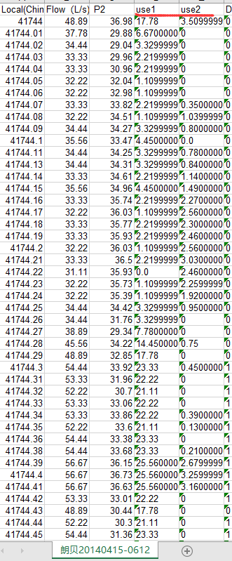

2 Typical Water Use Model

2.1 Unithermal Coding

This step maps the sample set to a Euclidean space for easy distance calculation, where the time characteristics are unithermal coded with constant water flow.

2.1.1 Mapping Date

def get_timeMap():
    data = xlrd.open_workbook("2018 Northeast Three Provinces Mathematical Modeling League in 1997 F Annex.xls")  # Open excel
    table = data.sheet_by_name("Lambert 20140 415-0612")  # Read sheet
    timeMap = {}
    for i in range(1, table.nrows):
        row = table.row_values(i)  # Line data in an array
        date = xldate_as_tuple(row[0], 0)
        if date[1] == 4 and date[2] == 15:
            key = str(date[3]) + ":" + str(date[4]) + ":" +str(date[5])
            timeMap[key] = i
    enc = preprocessing.OneHotEncoder()
    studyData = []
    for item in timeMap.values():
        studyData.append([item])
    enc.fit(studyData)  # fit to learn coding
    endcodeData = enc.transform(studyData).toarray().tolist()   # Coding
    count = 0
    for key in timeMap.keys():
        timeMap[key] = endcodeData[count]
        count = count + 1
    return timeMap

2.1.2 Coding Vector

A sample vector is constructed by combining the mapping date and water consumption.

timeMap = get_timeMap()
    data = xlrd.open_workbook("2018 Northeast Three Provinces Mathematical Modeling League F Annex.xls")  # Open excel
    table = data.sheet_by_name("Lambert 20140 415-0612")  # Read sheet
    vectors1 = []
    vectors2 = []
    for i in range(1, table.nrows):
        row = table.row_values(i)  # Line data in an array
        date = xldate_as_tuple(row[0], 0)
        key = str(date[3]) + ":" + str(date[4]) + ":" + str(date[5])
        item1 = copy.deepcopy(timeMap[key])         # Pay attention to deep replication
        item1.append(use1[i-1])
        vectors1.append(item1)
        item2 = copy.deepcopy(timeMap[key])
        item2.append(use2[i - 1])
        vectors2.append(item2)
    return np.array(vectors1), np.array(vectors2)

give the result as follows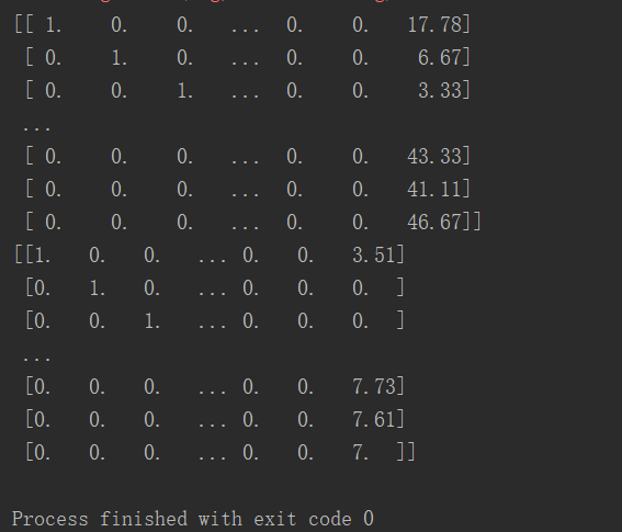

2.2 Cluster Evaluation

Take contour coefficient

def choose_by_silhouette(X):
    tests = [2, 3, 4, 5]
    sc_scores = []
    for k in tests:
        kmeans_model = KMeans(n_clusters=k).fit(X)
        sc_score = metrics.silhouette_score(X, kmeans_model.labels_, metric='euclidean')
        sc_scores.append(sc_score)
return sc_scores

The results of k taking 2, 3, 4 and 5 are as follows.

2.3 K Mean Classification

You need to retrieve the list of times before classifying, using the previous read_all() method, but you need to change the date in times to the same day.

 for count in range(0, len(times)):
         times[count] = times[count].replace(2014, 4, 15)

The parameters obtained before input can be classified.

def cluster_by_K(x1, x2, X, k, name):
    '''
    :param x1:   Time list
    :param x2:   Water consumption list
    :param X:    Matrix composed of sample vectors
    :param k:    k value
    :param name: Picture name
    :return:
    '''
    data = xlrd.open_workbook("result.xls")  # Open excel
    from xlutils.copy import copy
    wb = xlutils.copy.copy(data)
    sheet = wb.get_sheet(0)
    if name == 'DMA1':
        cloumn = 3
    else:
        cloumn = 4
    sheet.write(0, cloumn, name)
    plt.figure(figsize=(8, 6))
    colors = ['b', 'g', 'r', 'c', 'm', 'y', 'k', 'b']
    markers = ['o', 's', 'D', 'v', '^', 'p', '*', '+']
    kmeans_model = KMeans(n_clusters=k).fit(X)
    for i, l in enumerate(kmeans_model.labels_):
        plt.subplot(k, 1, 1 + l)
        sheet.write(i+1, cloumn, str(l))
        print(i)
        plt.plot(x1[i], x2[i], color=colors[l], marker=markers[l])
    wb.save("result.xls")
    for t in range(1, k+1):
        plt.subplot(k, 1, t)
        plt.gca().xaxis.set_major_formatter(mdates.DateFormatter('%H:%M:%S'))
        plt.gcf().autofmt_xdate()  # Automatic Rotation Date Marker
        plt.title('The first'+str(t)+'species', fontproperties=font)
    plt.savefig(name+'.png')
    return kmeans_model.labels_

The results of DMA1 are as follows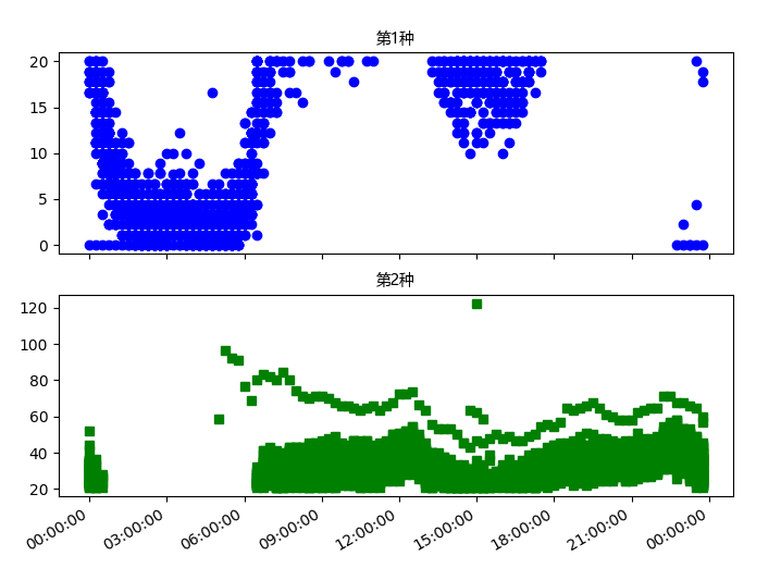

The results of DMA2 are as follows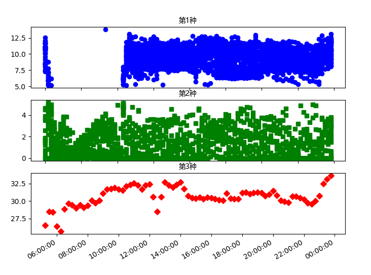

At the same time, the results are appended to the document for reuse.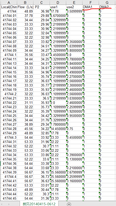

3. Abnormal pattern recognition

3.1 Extraction Characteristics

3.1.1 Calculating the Variation

def cal_change():
    data = xlrd.open_workbook("result.xls")  # Open excel
    table = data.sheet_by_name("Lambert 20140 415-0612")  # Read sheet
    from xlutils.copy import copy
    wb = xlutils.copy.copy(data)
    sheet = wb.get_sheet(0)
    sheet.write(0, 7, 'change1')
    sheet.write(0, 8, 'change2')
    oldRow = table.row_values(1)
    for i in range(2, table.nrows):
        row = table.row_values(i)  # Line data in an array
        sheet.write(i, 7, abs(float(row[3]) - float(oldRow[3])))
        sheet.write(i, 8, abs(float(row[4]) - float(oldRow[4])))
        oldRow = row
    wb.save("result.xls")

Append the calculated amount of change to the back of the document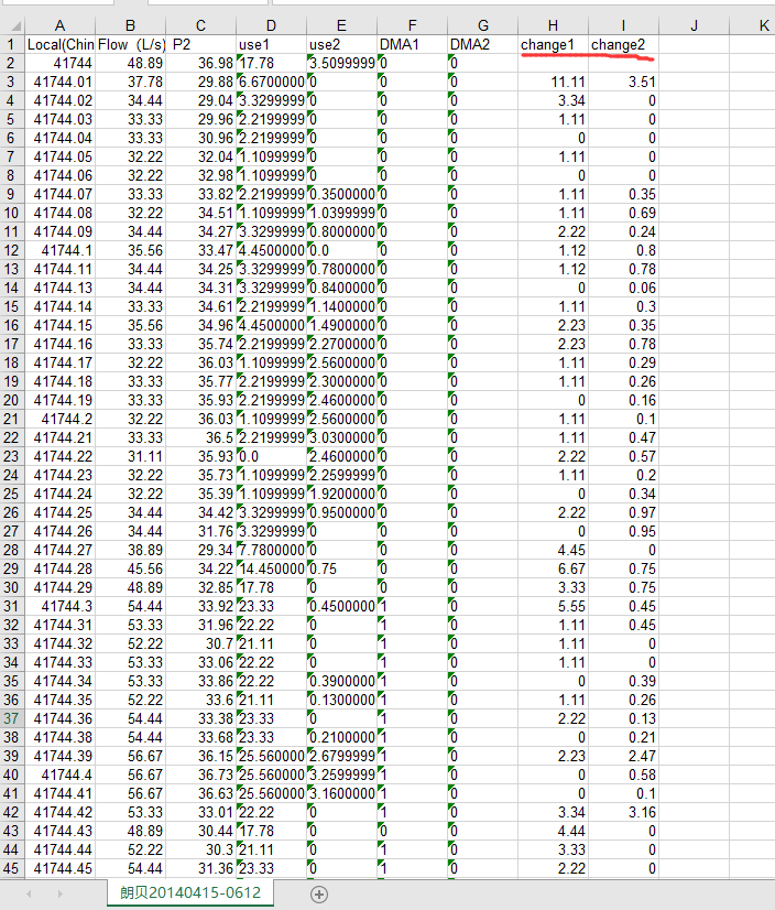

3.1.2 Construction Matrix

Constructing different matrices for clustering after different patterns

def get_change():
    data = xlrd.open_workbook("result.xls")  # Open excel
    table = data.sheet_by_name("Lambert 20140 415-0612")  # Read sheet
    DMA10 = []
    DMA11 = []
    DMA20 = []
    DMA21 = []
    DMA22 = []
    oldRow = table.row_values(1)
    for i in range(2, table.nrows):
        row = table.row_values(i)  # Line data in an array
        item = [float(row[3]), abs(float(row[3]) - float(oldRow[3]))]
        if int(row[5]) == 0:
            DMA10.append(item)
        else:
            DMA11.append(item)
        item = [float(row[4]), abs(float(row[4]) - float(oldRow[4]))]
        if int(row[6]) == 0:
            DMA20.append(item)
        elif int(row[6]) == 1:
            DMA21.append(item)
        else:
            DMA22.append(item)
        oldRow = row
    return np.array(DMA10), np.array(DMA11),np.array(DMA20), np.array(DMA21), np.array(DMA22)

3.2DBSCAN Clustering

After clustering, the distribution map of points is drawn according to the label value.

def find_by_DBSCAN(X, eps, min_samples, name):
    y_pred = DBSCAN(eps=eps, min_samples=min_samples).fit_predict(X)
    plt.scatter(X[:, 0], X[:, 1], c=y_pred)
    # plt.show()
    plt.savefig(name)

Remember to adjust the parameters for different types. I'll give you the case of mode 0 of DMA1 with eps=10 and min_samples=10 (corresponding to mode 1 in the original text).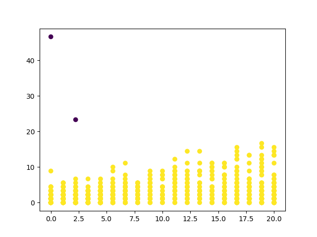

3.3 Print outliers

Call after clustering

def print_exception(lables, name):
    if name == "DMA10":
        columnIndex = 5
        typeValue = 0
    elif name == "DMA11":
        columnIndex = 5
        typeValue = 1
    elif name == "DMA20":
        columnIndex = 6
        typeValue = 0
    elif name == "DMA21":
        columnIndex = 6
        typeValue = 1
    elif name == "DMA22":
        columnIndex = 6
        typeValue = 2
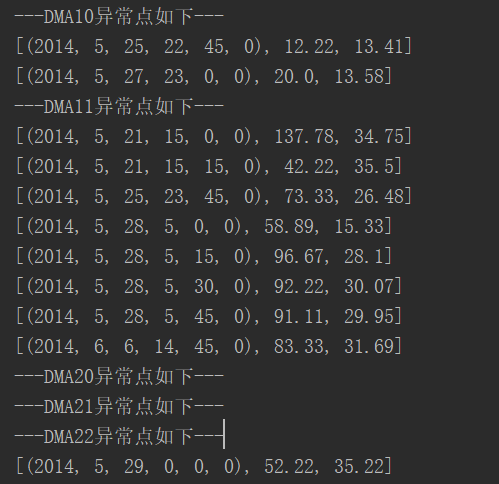
    print("---"+name+"The outliers are as follows---")
    data = xlrd.open_workbook("result.xls")  # Open excel
    table = data.sheet_by_name("Lambert 20140 415-0612")  # Read sheet
    count = 0
    for i in range(2, table.nrows):
        row = table.row_values(i)  # Line data in an array
        if int(row[columnIndex]) == int(typeValue):
            count = count + 1
            if int(lables[count - 1]) != 0:
                date = xldate_as_tuple(row[0], 0)
                print([date, row[1], row[2]])

It can be seen that the results are not very different from those given in the paper. It should be noted that my 0 and 1 are exactly opposite to the model 0 and 1 of the paper.