Chapter 9 Start and Run TensorFlow
Proofreading: @Lisanaaa @Flydragon
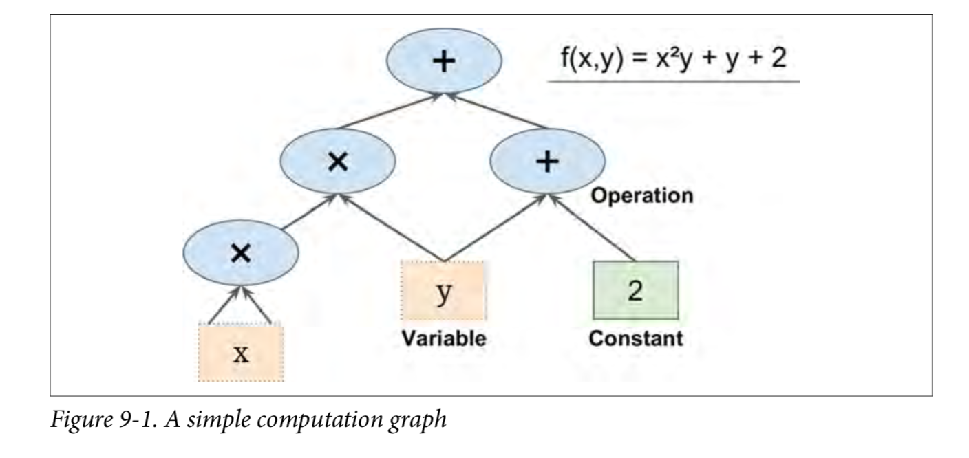
TensorFlow is a powerful open source software library for numerical computing, especially for fine-tuning of large-scale machine learning.Its basic principle is simple: first define the calculation diagram to be executed in Python (for example, Figure 9-1), then TensorFlow uses the diagram and runs it efficiently using optimized C++ code.
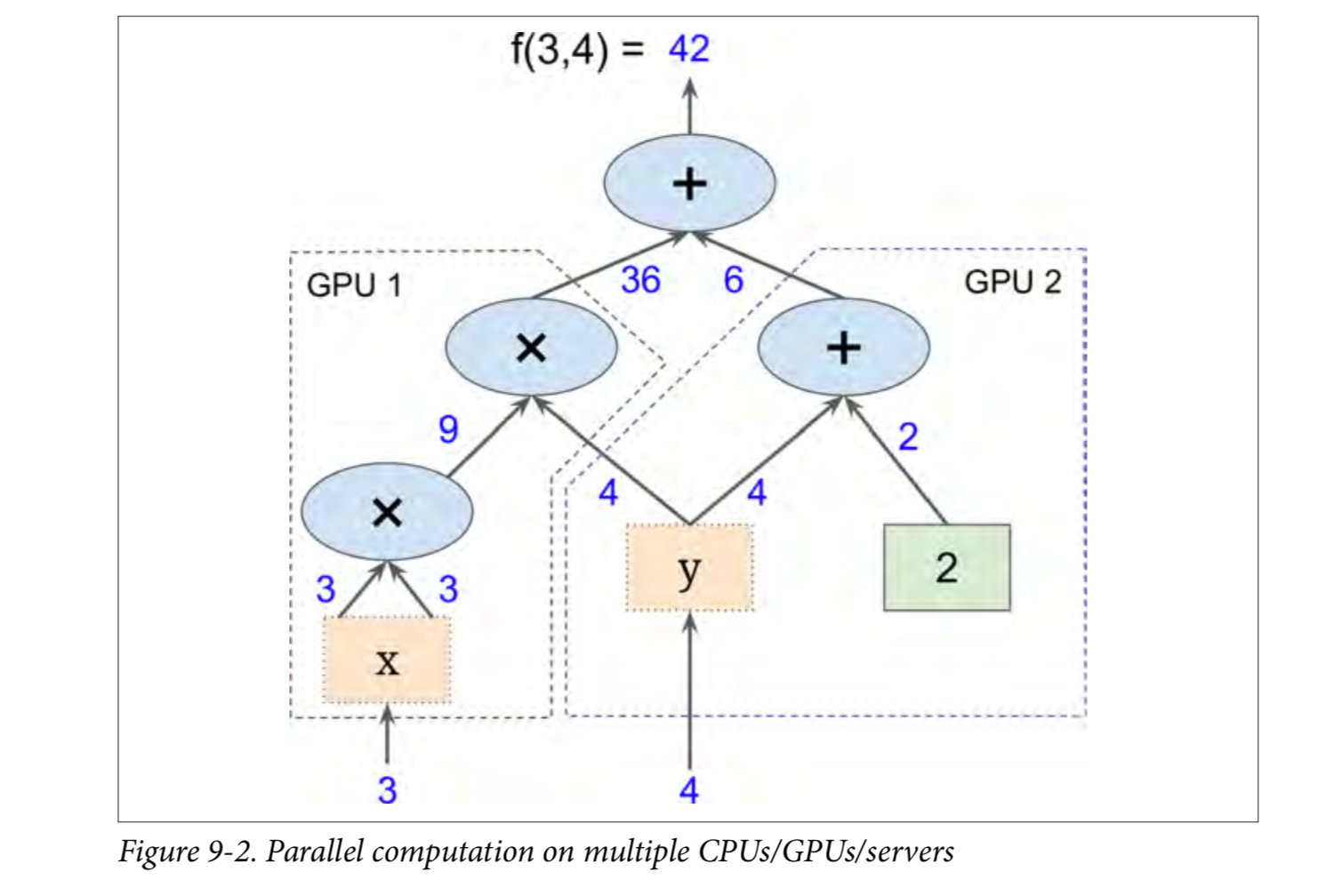
Most importantly, Tensorflow can decompose the graph into blocks and run parallel across multiple CPU s or GPU s (as shown in Figures 9-2).TensorFlow also supports distributed computing, so you can split the computing across hundreds of servers to train large neural networks over large training sets in a reasonable amount of time (see chapter 12).TensorFlow can train a network with millions of parameters, and the training set consists of billions of instances with millions of features.This shouldn't surprise you, because TensorFlow was developed by the Google Brain Team and supports a number of Google services, such as Google Cloud Speech, Google Photos, and Google Search.
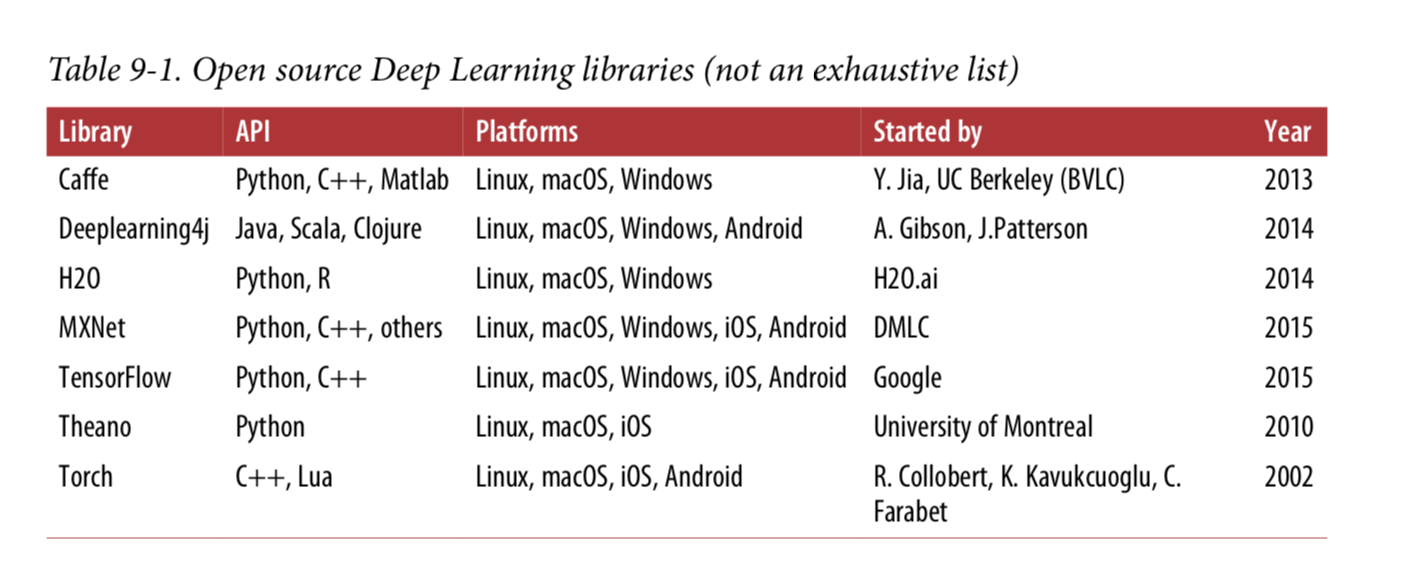
When TensorFlow opened source code in November 2015, there were many popular open source libraries for in-depth learning (some listed in tables 9-1), fairly speaking, most of the TensorFlow functionality already exists in one library or another.Nevertheless, TensorFlow's clean design, scalability, flexibility and excellent documentation (not to mention Google's name) quickly pushed it to the top.In short, TensorFlow is designed for flexibility, scalability, and production readiness, and only three of the existing frameworks are available.Here are some highlights of TensorFlow:
-
It runs not only on Windows, Linux, and MacOS, but also on mobile devices, including iOS and Android.
It provides a very simple Python API called TF.Learn2 (tensorflow.con trib.learn), which is compatible with Scikit-Learn.As you will see, you can use a few lines of code to train different types of neural networks.Previously, it was a stand-alone project called Scikit Flow (or Skow).
It also provides another simple API called TF-slim (tensorflow.contrib.slim) to simplify building, training and deriving neural networks.
Several other advanced API s have been independently built on top of TensorFlow, such as Keras or Pretty Tensor.
Its main Python API provides more flexibility (at the expense of greater complexity) to create calculations, including any neural network structure you can think of.
It includes efficient C++ implementations of many ML operations, especially C++ implementations needed to build neural networks.There is also a C++ API to define your own high-performance operations.
It provides several advanced optimization nodes to search for parameters that minimize the loss function.These are very easy to use because TensorFlow automatically handles calculating gradients for the functions you define.This is called automatic decomposition (or autodi).
It also comes with a powerful visualization tool called TensorBoard that lets you browse calculation charts, view learning curves, and more.
Google also introduced a cloud service to run TensorFlow tables.
Finally, it has a passionate and helpful development team and a growing community dedicated to improving it.It's one of the most popular open source projects on GitHub, and more and more great projects are being built (for example, view https://www.tensorflow.org/ or https://github.com/jtoy/awesome-tensorflow ).To ask technical questions, you should use http://stackoverflow.com/ And tag your question with tensorflow.You can submit errors and feature requests through GitHub.For general discussion, join the Google group.
In this chapter, we will introduce the basics of TensorFlow, from installation to creation, running, saving and visualizing simple computational diagrams.It is important to have these basics before building the first neural network (we will cover them in the next chapter).
install
Let's get started!Assuming you have installed Jupyter and Scikit-Learn following the installation instructions in Chapter 2, you can simply install TensorFlow using pip.If you create a separate environment using virtualenv, you first need to activate it:
$ cd $ML_PATH                            #Your ML working directory(e.g., $HOME/ml``)
$ source env/bin/activate
Next, install Tensorflow.
$ pip3 install --upgrade tensorflow
For GPU support, you need to install tensorflow-gpu instead of tensorflow.See Chapter 12 for details.
To test your installation, enter a command.The output should be the version number of the Tensorflow you installed.
$ python -c 'import tensorflow; print(tensorflow.__version__)'
1.0.0
Create the first map and run it
import tensorflow as tf
x = tf.Variable(3, name="x")
y = tf.Variable(4, name="y")
f = x*x*y + y + 2
$ cd $ML_PATH                            #Your ML working directory(e.g., $HOME/ml``)
That's it all!The most important thing to know is that this code does not actually perform any calculations, even if it looks like (especially on the last line).It just creates a computed graph.In fact, none of the variables are initialized. To get this diagram, you need to open a TensorFlow session and use it to initialize the variables and find F.The TensorFlow session handles and runs operations on devices such as CPU s and GPU s, and it retains all variable values.The following code creates a session, initializes variables, evaluates f, and closes the session (frees up resources):
# way1
sess = tf.Session()
sess.run(x.initializer)
sess.run(y.initializer)
result = sess.run(f)

print(result)
sess.close()
Having to repeat sess.run() every time is a little cumbersome, but fortunately there is a better way:
# way2
with tf.Session() as sess:
    x.initializer.run()
    y.initializer.run()
    result = f.eval()
print(result)
In the with block, the session is set as the default session.Calling x.initializer.run() is equivalent to calling tf.get_default_session().run(x.initial), and f.eval() is equivalent to calling tf.get_default_session().run(f).This makes the code easier to read.In addition, the session is automatically closed at the end of the block.
Instead of initializing each variable manually, you can use the global_variables_initializer() function.Note that instead of actually initializing immediately, it creates a node in the spectrum that all variables initialize when the program runs:
# way3
# init = tf.global_variables_initializer()
# with tf.Session() as sess:
#     init.run()
#     result = f.eval()
6. # print(result)
Inside Jupyter or in the Python shell, you may prefer to create an Interactive Session.The only difference with regular sessions is that when an Interactive Session is created, it automatically sets itself as the default session, so you don't need to use a module (but you need to close the session manually when you're finished):
# way4
init = tf.global_variables_initializer()
sess = tf.InteractiveSession()
init.run()
result = f.eval()
print(result)
sess.close()
The TensorFlow program is usually divided into two parts: the first part builds the computational map (called the construction phase) and the second part runs it (this is the execution phase).In the construction phase, a computational map representing the ML model is usually constructed, then trained and calculated.The execution phase typically runs a loop, repeatedly calculating training steps (for example, each small batch) and gradually improving the model parameters.
Management Map
Any node you create is automatically added to the default graph:
>>> x1 = tf.Variable(1)
>>> x1.graph is tf.get_default_graph()
True
In most cases, this is good, but sometimes you may need to manage multiple independent graphics.You can create a new graphic and temporarily set it as the default graphic in a block, as follows:
>>> graph = tf.Graph()
>>> with graph.as_default():
... x2 = tf.Variable(2)
...
>>> x2.graph is graph
True
>>> x2.graph is tf.get_default_graph()
False
In Jupyter (or Python shell), it is common to run the same command multiple times during an experiment.Therefore, you may receive a default graph containing many duplicate nodes.One solution is to restart the Jupyter kernel (or Python shell), but a more convenient solution is to reset the default graph by running tf.reset_default_graph().
Life cycle of node value
When nodes are found, TensorFlow automatically determines the set of nodes it depends on and first evaluates them.For example, consider the following code:
# w = tf.constant(3)
# x = w + 2
# y = x + 5
# z = x * 3

# with tf.Session() as sess:
#     print(y.eval())
#     print(z.eval())
First, the code defines a very simple graph.It then starts a session and runs the graph to find that y:TensorFlow automatically detects y dependent on X and it depends on w, so it first evaluates w, then x, then y, and returns the value of Y.Finally, the code runs through the diagram to find the z.Similarly, TensorFlow detects that it must first find w and X.It is important to note that it does not reuse previous W and X results.In short, the preceding code evaluates W and X twice.
All node values are deleted between graph runs and are maintained by the session across the graph except for variable values (queues and readers remain in some state).A variable starts its life cycle when its initializer runs and ends when the session closes.
If you want to find y and z effectively instead of w and x twice as in the previous code, you must ask TensorFlow to find y and z in a graph run, as shown in the following code:
# with tf.Session() as sess:
#     y_val, z_val = sess.run([y, z])
#     print(y_val) # 10
#     print(z_val) # 15
In a single-process TensorFlow, multiple sessions do not share any state, even if they reuse the same graph (each session has its own copy of each variable).In distributed TensorFlow, variable state is stored on the server, not in the session, so multiple sessions can share the same variable.
Linear Regression with TensorFlow
The TensorFlow operation (also referred to as ops) can take any number of inputs and produce any number of outputs.For example, addition and multiplication require two inputs and produce one output.Constants and variables are not entered (they are called source operations).The input and output are multidimensional arrays called tensors (hence "tensor flow").Like NumPy arrays, tensors have types and shapes.In fact, in the Python API, tensors are simply represented by NumPyndarray.They usually contain floating-point numbers, but you can also use them to transfer strings (any byte array).
In the example so far, a tensor contains only a single scalar value, but of course you can perform calculations on arrays of any shape.For example, the following code manipulates a two-dimensional array to perform linear regression on a California housing dataset (described in chapter 2).It starts by getting the dataset; then it adds an additional offset input feature (x0 = 1) to all training instances (it runs immediately because it uses NumPy); then it creates two TensorFlow constant nodes X and y to hold the data and the target, and it uses some of the matrix operations provided by TensorFlow to define the theta.These matrix functions transpose(), matmul(), and matrix_inverse() are self-explanatory, but as always, they do not perform any calculations immediately; instead, they create nodes in the graph that execute them when the graph is run.You can recognize that the definition of theta corresponds to the equation
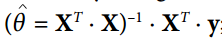
Finally, the code creates a session and uses it to find the theta.
import numpy as np
from sklearn.datasets import fetch_california_housing
housing = fetch_california_housing()
m, n = housing.data.shape
#np.c_Combine array s by colunm
housing_data_plus_bias = np.c_[np.ones((m, 1)), housing.data]

X = tf.constant(housing_data_plus_bias, dtype=tf.float32, name="X")
y = tf.constant(housing.target.reshape(-1, 1), dtype=tf.float32, name="y")
XT = tf.transpose(X)
theta = tf.matmul(tf.matmul(tf.matrix_inverse(tf.matmul(XT, X)), XT), y)
with tf.Session() as sess:
    theta_value = theta.eval()
print(theta_value)
If you have a GPU, the main advantage of the above code over calculating normal equations directly using NumPy is that TensorFlow runs automatically on your GPU (if you install a TensorFlow that supports GPU, TensorFlow runs automatically on the GPU, see Chapter 12 for more details).
In fact, this is the least squares method for calculating theta
http://blog.csdn.net/akon_wang_hkbu/article/details/77503725
Achieving Gradient Decrease
Let's try using batch gradient descent (described in chapter 4) instead of the general equation.First, we'll calculate the gradient manually, then we'll use the automatic extension of TensorFlow to make TensorFlow automatically calculate the gradient, and finally we'll use several TensorFlow optimizers.
When using gradient descent, remember to first normalize the input eigenvectors, otherwise the training may be much slower.You can use TensorFlow, NumPy, Scikit-Learn Standaard Scaler or any other solution you like.The following code assumes that this normalization has been completed.
Manually calculate gradients
The following code should be fairly self-explanatory, except for a few new elements:
- The random_uniform() function creates a node in the graph that generates a tensor containing random values, given its shape and range of values, just like NumPy's rand() function.
- The assign() function creates a node that assigns a new value to a variable.In this case, it implements the batch gradient descent step $\theta(next step)= \theta - \eta \nabla_{\theta}MSE(\theta)$.
- The main loop executes the training steps again and again (n_epochs in total), printing out the current mean square error (MSE) every 100 iterations.You should see that the MSE decreases in each iteration.
housing = fetch_california_housing()
m, n = housing.data.shape
m, n = housing.data.shape
#np.c_Combine array s by colunm
housing_data_plus_bias = np.c_[np.ones((m, 1)), housing.data]
scaled_housing_data_plus_bias = scale(housing_data_plus_bias)
n_epochs = 1000
learning_rate = 0.01
X = tf.constant(scaled_housing_data_plus_bias, dtype=tf.float32, name="X")
y = tf.constant(housing.target.reshape(-1, 1), dtype=tf.float32, name="y")
theta = tf.Variable(tf.random_uniform([n + 1, 1], -1.0, 1.0), name="theta")
y_pred = tf.matmul(X, theta, name="predictions")
error = y_pred - y
mse = tf.reduce_mean(tf.square(error), name="mse")
gradients = 2/m * tf.matmul(tf.transpose(X), error)
training_op = tf.assign(theta, theta - learning_rate * gradients)
init = tf.global_variables_initializer()
with tf.Session() as sess:
    sess.run(init)
    for epoch in range(n_epochs):
        if epoch % 100 == 0:
            print("Epoch", epoch, "MSE =", mse.eval())
        sess.run(training_op)
    best_theta = theta.eval()
Using autodiff
The previous code works fine, but it requires a mathematical formula to derive the gradient from the cost function (MSE).In the case of linear regression, this is fairly easy, but if you have to do it with deep neural networks, you will experience headaches: it will be tedious and error prone.You can use symbolic derivatives to automatically find equations for partial derivatives for you, but the resulting code may not be very effective.
To understand why, consider the function f(x) = exp(exp(x)).If you know a calculus, you can calculate its derivative f'(x) = exp(x) * exp(x) * exp(x) * exp(x)).If you write f(x) and f'(x) separately in the normal way of calculation, your code will not be so effective.A more efficient solution is to write a function that first evaluates exp(x), then exp(x), then exp(exp(x)) and returns all three.This gives you (third item) f(x) directly. If you need to derive, you can multiply the three Sub-Formulas and you are done.Traditionally, you have to call the exp function nine times to calculate f(x) and f'(x).In this way, you only need to call it three times.
When your function is defined by some arbitrary code, it gets worse.Can you find the equation (or code) to calculate the partial derivatives of the following functions?
Tip: Don't try.
def my_func(a, b):
    z = 0
    for i in range(100):
        z = a * np.cos(z + i) + z * np.sin(b - i)
    return z
Fortunately, TensorFlow's automatic gradient calculation function calculates this formula: it automatically and efficiently calculates gradients for you.Simply replace the gradients =... Line of the code in the previous section with the following line of code, and the code will continue to work correctly:
gradients = tf.gradients(mse, [theta])[0]
The gradients() function uses an op (MSE in this case) and a list of variables (theta in this case) to create an ops list (one for each variable) to calculate the gradient variable for Op.Therefore, the gradient nodes will compute the MSE gradient vector relative to theta.
There are four main methods for automatically calculating gradients.They are summarized in tables 9-2.TensorFlow uses the reverse mode, which is perfect (efficient and accurate) when there are many inputs and a small number of outputs, such as in the case of neural networks.It only needs $n_{outputs} + 1$graph traversal to calculate the partial derivatives of all outputs.
update statistics
So TensorFlow calculates the gradient for you.But there is a better way: it also provides some optimizers that can be used directly, including the Gradient Down optimizer.You can simply replace the previous gradients =... And training_op =... Lines with the following code, and everything will work:
optimizer = tf.train.GradientDescentOptimizer(learning_rate=learning_rate)
training_op = optimizer.minimize(mse)
If you want to use another type of optimizer, you only need to change one line.For example, you can use a momentum optimizer by defining an optimizer (usually converges much faster than a gradual convergence; see Chapter 11)
optimizer = tf.train.MomentumOptimizer(learning_rate=learning_rate, momentum=0.9)
Providing data to training algorithms
We tried to modify the previous code to achieve a small batch gradient descent (Mini-batch Gradient Descent).To do this, we need a way to replace X and Y with the next small batch at each iteration.The easiest way is to use placeholder nodes.These nodes are special because they don't actually perform any calculations, they just output the data you output at run time.They are often used to transfer training data to TensorFlow during training.If no value is specified for the placeholder at runtime, an exception is received.
To create a placeholder node, you must call the placeholder() function and specify the data type of the output tensor.Alternatively, you can specify its shape, if enforced.If the specified dimension is None, it means "any size".For example, the following code creates a placeholder node A and a node B = A + 5.When we find B, we pass a feed_dict to the eval() method and specify the value of A.Note that A must have level 2 (that is, it must be two-dimensional), and must have three columns (otherwise an exception is thrown), but it can have any number of rows.
>>> A = tf.placeholder(tf.float32, shape=(None, 3))
>>> B = A + 5
>>> with tf.Session() as sess:
... B_val_1 = B.eval(feed_dict={A: [[1, 2, 3]]})
... B_val_2 = B.eval(feed_dict={A: [[4, 5, 6], [7, 8, 9]]})
...
>>> print(B_val_1)
[[ 6. 7. 8.]]
>>> print(B_val_2)
[[ 9. 10. 11.]
[ 12. 13. 14.]]
You can actually provide output for any operation, not just placeholders.In this case, TensorFlow does not attempt to find out these operations; it uses the value you provide.
To achieve small batch gradients, we only need to adjust the existing code a little.First change the definitions of X and Y to define them as placeholder nodes:
X = tf.placeholder(tf.float32, shape=(None, n + 1), name="X")
y = tf.placeholder(tf.float32, shape=(None, 1), name="y")
Then define the batch size and calculate the total number of batches:
batch_size = 100
n_batches = int(np.ceil(m / batch_size))
Finally, in the execution phase, small batches are obtained one by one, and then X and y values are provided through feed_dict when any node that relies on X and y values is evaluated.
def fetch_batch(epoch, batch_index, batch_size):
    [...] # load the data from disk
    return X_batch, y_batch

with tf.Session() as sess:
    sess.run(init)

    for epoch in range(n_epochs):
        for batch_index in range(n_batches):
            X_batch, y_batch = fetch_batch(epoch, batch_index, batch_size)
            sess.run(training_op, feed_dict={X: X_batch, y: y_batch})
    best_theta = theta.eval()
When calculating the theta, we don't need to pass the values of X and y because it doesn't depend on them.
MINI-BATCH full code
import numpy as np
from sklearn.datasets import fetch_california_housing
import tensorflow as tf
from sklearn.preprocessing import StandardScaler

housing = fetch_california_housing()
m, n = housing.data.shape
print("data set:{}That's ok,{}column".format(m,n))
housing_data_plus_bias = np.c_[np.ones((m, 1)), housing.data]
scaler = StandardScaler()
scaled_housing_data = scaler.fit_transform(housing.data)
scaled_housing_data_plus_bias = np.c_[np.ones((m, 1)), scaled_housing_data]

n_epochs = 1000
learning_rate = 0.01

X = tf.placeholder(tf.float32, shape=(None, n + 1), name="X")
y = tf.placeholder(tf.float32, shape=(None, 1), name="y")
theta = tf.Variable(tf.random_uniform([n + 1, 1], -1.0, 1.0, seed=42), name="theta")
y_pred = tf.matmul(X, theta, name="predictions")
error = y_pred - y
mse = tf.reduce_mean(tf.square(error), name="mse")
optimizer = tf.train.GradientDescentOptimizer(learning_rate=learning_rate)
training_op = optimizer.minimize(mse)

init = tf.global_variables_initializer()

n_epochs = 10
batch_size = 100
n_batches = int(np.ceil(m / batch_size)) # The ceil() method returns the upper limit of the value of X - the smallest integer that is no less than x.

def fetch_batch(epoch, batch_index, batch_size):
    know = np.random.seed(epoch * n_batches + batch_index)  # not shown in the book
    print("I am know:",know)
    indices = np.random.randint(m, size=batch_size)  # not shown
    X_batch = scaled_housing_data_plus_bias[indices] # not shown
    y_batch = housing.target.reshape(-1, 1)[indices] # not shown
    return X_batch, y_batch

with tf.Session() as sess:
    sess.run(init)

    for epoch in range(n_epochs):
        for batch_index in range(n_batches):
            X_batch, y_batch = fetch_batch(epoch, batch_index, batch_size)
            sess.run(training_op, feed_dict={X: X_batch, y: y_batch})

    best_theta = theta.eval()

print(best_theta)
Save and restore models
Once you've trained your model, you should save its parameters to disk, so you can go back to it anytime, anywhere, use it in another program, compare it with other models, and so on.In addition, you may want to save checkpoints periodically during training so that if your computer crashes during training, you can continue from the last checkpoint instead of starting from scratch.
TensorFlow makes it easy to save and restore models.Simply create a save node at the end of the construction phase (after all variable nodes have been created); then, in the execution phase, call its save() method whenever you want to save the model:
[...]
theta = tf.Variable(tf.random_uniform([n + 1, 1], -1.0, 1.0), name="theta")
[...]
init = tf.global_variables_initializer()
saver = tf.train.Saver()
with tf.Session() as sess:
    sess.run(init)

    for epoch in range(n_epochs):
        if epoch % 100 == 0: # checkpoint every 100 epochs
            save_path = saver.save(sess, "/tmp/my_model.ckpt")

        sess.run(training_op)
    best_theta = theta.eval()
    save_path = saver.save(sess, "/tmp/my_model_final.ckpt")
Restoring a model is as easy as creating a saver at the end of the build phase as before, but at the beginning of the execution phase, instead of initializing variables with init nodes, you can call the saver object of the restore() method:
with tf.Session() as sess:
    saver.restore(sess, "/tmp/my_model_final.ckpt")
    [...]
By default, the saver saves and restores all variables with its own name, but if more control is needed, you can specify the variables to save or restore and the name to use.For example, the following saver will save or restore only the theta variable, whose key name is weights:
saver = tf.train.Saver({"weights": theta})
Complete Code
 numpy as np
from sklearn.datasets import fetch_california_housing
import tensorflow as tf
from sklearn.preprocessing import StandardScaler

housing = fetch_california_housing()
m, n = housing.data.shape
print("data set:{}That's ok,{}column".format(m,n))
housing_data_plus_bias = np.c_[np.ones((m, 1)), housing.data]
scaler = StandardScaler()
scaled_housing_data = scaler.fit_transform(housing.data)
scaled_housing_data_plus_bias = np.c_[np.ones((m, 1)), scaled_housing_data]

n_epochs = 1000  # not shown in the book
learning_rate = 0.01  # not shown

X = tf.constant(scaled_housing_data_plus_bias, dtype=tf.float32, name="X")  # not shown
y = tf.constant(housing.target.reshape(-1, 1), dtype=tf.float32, name="y")  # not shown
theta = tf.Variable(tf.random_uniform([n + 1, 1], -1.0, 1.0, seed=42), name="theta")
y_pred = tf.matmul(X, theta, name="predictions")  # not shown
error = y_pred - y  # not shown
mse = tf.reduce_mean(tf.square(error), name="mse")  # not shown
optimizer = tf.train.GradientDescentOptimizer(learning_rate=learning_rate)  # not shown
training_op = optimizer.minimize(mse)  # not shown

init = tf.global_variables_initializer()
saver = tf.train.Saver()

with tf.Session() as sess:
    sess.run(init)

    for epoch in range(n_epochs):
        if epoch % 100 == 0:
            print("Epoch", epoch, "MSE =", mse.eval())  # not shown
            save_path = saver.save(sess, "/tmp/my_model.ckpt")
        sess.run(training_op)

    best_theta = theta.eval()
    save_path = saver.save(sess, "/tmp/my_model_final.ckpt") #Find the tmp folder and the file
Use TensorBoard to display graphics and training curves
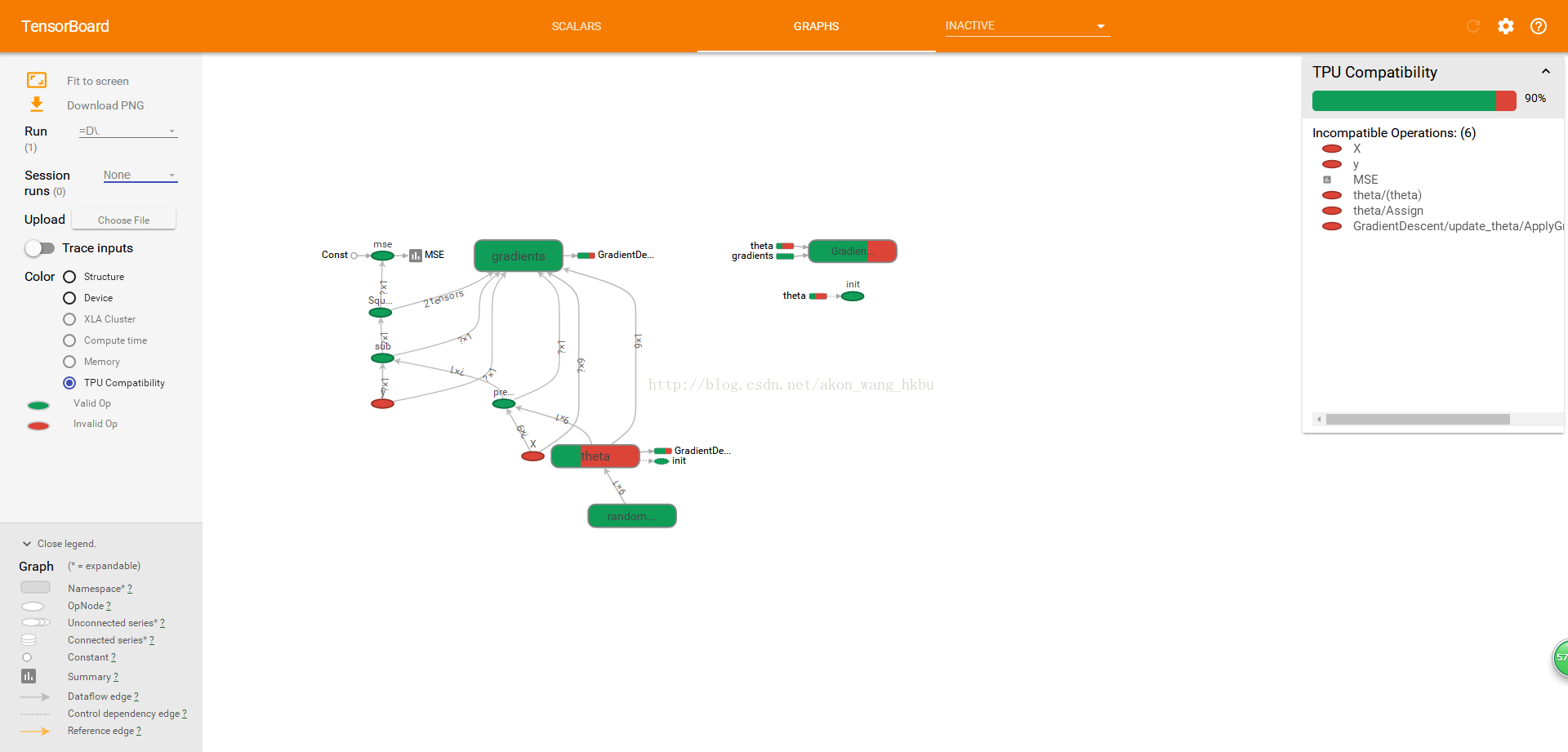
So now we have a computed map of a linear regression model trained with small batch gradient descent, and we are periodically saving checkpoints.Sounds complicated, doesn't it?However, we still rely on the print() function to visualize the progress of the training process.A better way to do this is to enter the TensorBoard.If you provide some training statistics, it will display a good interactive visualization of these statistics (such as learning curves) in your web browser.You can also provide a definition of a graphic, which provides a good interface for you to browse through it.This can be useful for identifying errors in diagrams, finding bottlenecks, and so on.
The first step is to adjust the program so that the graphical definition and some training statistics (for example, training_error (MSE)) are written to the log directory TensorBoard will read.You need to use a different log directory each time you run the program, or TensorBoard will merge statistics from different runs, which will confuse visualization.The simplest solution is to include a time stamp in the log directory name.Add the following code at the beginning of the program:
from datetime import datetime
now = datetime.utcnow().strftime("%Y%m%d%H%M%S")
root_logdir = "tf_logs"
logdir = "{}/run-{}/".format(root_logdir, now)
Next, add the following code at the end of the build phase:
mse_summary = tf.summary.scalar('MSE', mse)
file_writer = tf.summary.FileWriter(logdir, tf.get_default_graph())
The first line creates a node that evaluates the MSE value and writes it to a TensorBoard-compatible binary log string called a summary.The second line creates a FileWriter that you will use to write a summary to a log file in the log directory.The first parameter indicates the path to the log directory (in this case tf_logs/run-20160906091959/, relative to the current directory).The second (optional) parameter is the graphic you want to visualize.When created, the file writer creates a log directory (if needed) and defines it in a binary log file called an event file.
Next, you need to update the execution phase to periodically find the mse_summary nodes during training (for example, every 10 small batches).This outputs a summary, which can then be written to the event file using file_writer.Here is the updated code:
[...]
for batch_index in range(n_batches):
    X_batch, y_batch = fetch_batch(epoch, batch_index, batch_size)
    if batch_index % 10 == 0:
        summary_str = mse_summary.eval(feed_dict={X: X_batch, y: y_batch})
        step = epoch * n_batches + batch_index
        file_writer.add_summary(summary_str, step)
    sess.run(training_op, feed_dict={X: X_batch, y: y_batch})
[...]
Avoid recording training data at each training stage, as this will significantly slow down the training speed (the above code is recorded every 10 small batches).
Finally, close FileWriter at the end of the program:
file_writer.close()
Complete Code
import numpy as np
from sklearn.datasets import fetch_california_housing
import tensorflow as tf
from sklearn.preprocessing import StandardScaler

housing = fetch_california_housing()
m, n = housing.data.shape
print("data set:{}That's ok,{}column".format(m,n))
housing_data_plus_bias = np.c_[np.ones((m, 1)), housing.data]
scaler = StandardScaler()
scaled_housing_data = scaler.fit_transform(housing.data)
scaled_housing_data_plus_bias = np.c_[np.ones((m, 1)), scaled_housing_data]

from datetime import datetime

now = datetime.utcnow().strftime("%Y%m%d%H%M%S")
root_logdir = r"D://tf_logs"
logdir = "{}/run-{}/".format(root_logdir, now)
n_epochs = 1000
learning_rate = 0.01

X = tf.placeholder(tf.float32, shape=(None, n + 1), name="X")
y = tf.placeholder(tf.float32, shape=(None, 1), name="y")
theta = tf.Variable(tf.random_uniform([n + 1, 1], -1.0, 1.0, seed=42), name="theta")
y_pred = tf.matmul(X, theta, name="predictions")
error = y_pred - y
mse = tf.reduce_mean(tf.square(error), name="mse")
optimizer = tf.train.GradientDescentOptimizer(learning_rate=learning_rate)
training_op = optimizer.minimize(mse)

init = tf.global_variables_initializer()
mse_summary = tf.summary.scalar('MSE', mse)
file_writer = tf.summary.FileWriter(logdir, tf.get_default_graph())

n_epochs = 10
batch_size = 100
n_batches = int(np.ceil(m / batch_size))

def fetch_batch(epoch, batch_index, batch_size):
    np.random.seed(epoch * n_batches + batch_index)  # not shown in the book
    indices = np.random.randint(m, size=batch_size)  # not shown
    X_batch = scaled_housing_data_plus_bias[indices] # not shown
    y_batch = housing.target.reshape(-1, 1)[indices] # not shown
    return X_batch, y_batch

with tf.Session() as sess:                                                        # not shown in the book
    sess.run(init)                                                                # not shown

    for epoch in range(n_epochs):                                                 # not shown
        for batch_index in range(n_batches):
            X_batch, y_batch = fetch_batch(epoch, batch_index, batch_size)
            if batch_index % 10 == 0:
                summary_str = mse_summary.eval(feed_dict={X: X_batch, y: y_batch})
                step = epoch * n_batches + batch_index
                file_writer.add_summary(summary_str, step)
            sess.run(training_op, feed_dict={X: X_batch, y: y_batch})

    best_theta = theta.eval()
file_writer.close()
print(best_theta)
Name Scope
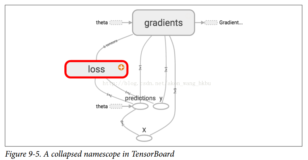
When dealing with more complex models, such as neural networks, the graph can easily be confused with thousands of nodes.To avoid this situation, you can create name scopes to group related nodes.For example, we modified the previous code to define errors and mse operations within the name scope named loss:
with tf.name_scope("loss") as scope:
    error = y_pred - y
    mse = tf.reduce_mean(tf.square(error), name="mse")
The name of each op defined within the scope is now prefixed with loss/
>>> print(error.op.name)
loss/sub
>>> print(mse.op.name)
loss/mse
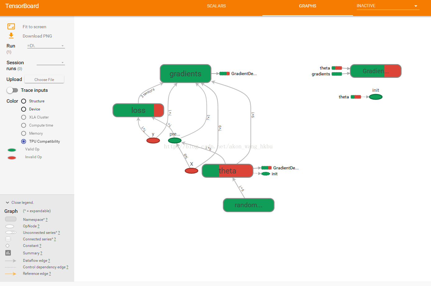
In TensorBoard, the mse and error nodes now appear in the loss namespace and crash by default (Figures 9-5).
Complete Code
import numpy as np
from sklearn.datasets import fetch_california_housing
import tensorflow as tf
from sklearn.preprocessing import StandardScaler

housing = fetch_california_housing()
m, n = housing.data.shape
print("data set:{}That's ok,{}column".format(m,n))
housing_data_plus_bias = np.c_[np.ones((m, 1)), housing.data]
scaler = StandardScaler()
scaled_housing_data = scaler.fit_transform(housing.data)
scaled_housing_data_plus_bias = np.c_[np.ones((m, 1)), scaled_housing_data]

from datetime import datetime

now = datetime.utcnow().strftime("%Y%m%d%H%M%S")
root_logdir = r"D://tf_logs"
logdir = "{}/run-{}/".format(root_logdir, now)

n_epochs = 1000
learning_rate = 0.01

X = tf.placeholder(tf.float32, shape=(None, n + 1), name="X")
y = tf.placeholder(tf.float32, shape=(None, 1), name="y")
theta = tf.Variable(tf.random_uniform([n + 1, 1], -1.0, 1.0, seed=42), name="theta")
y_pred = tf.matmul(X, theta, name="predictions")

def fetch_batch(epoch, batch_index, batch_size):
    np.random.seed(epoch * n_batches + batch_index)  # not shown in the book
    indices = np.random.randint(m, size=batch_size)  # not shown
    X_batch = scaled_housing_data_plus_bias[indices] # not shown
    y_batch = housing.target.reshape(-1, 1)[indices] # not shown
    return X_batch, y_batch

with tf.name_scope("loss") as scope:
    error = y_pred - y
    mse = tf.reduce_mean(tf.square(error), name="mse")

optimizer = tf.train.GradientDescentOptimizer(learning_rate=learning_rate)
training_op = optimizer.minimize(mse)

init = tf.global_variables_initializer()

mse_summary = tf.summary.scalar('MSE', mse)
file_writer = tf.summary.FileWriter(logdir, tf.get_default_graph())

n_epochs = 10
batch_size = 100
n_batches = int(np.ceil(m / batch_size))

with tf.Session() as sess:
    sess.run(init)

    for epoch in range(n_epochs):
        for batch_index in range(n_batches):
            X_batch, y_batch = fetch_batch(epoch, batch_index, batch_size)
            if batch_index % 10 == 0:
                summary_str = mse_summary.eval(feed_dict={X: X_batch, y: y_batch})
                step = epoch * n_batches + batch_index
                file_writer.add_summary(summary_str, step)
            sess.run(training_op, feed_dict={X: X_batch, y: y_batch})

    best_theta = theta.eval()

file_writer.flush()
file_writer.close()
print("Best theta:")
print(best_theta)
Modularity
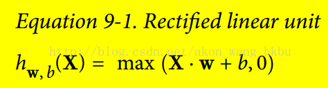
Suppose you want to create a graph that adds the output values of two rectifier linear units (ReLUs).ReLU calculates the output value of a corresponding linear function of an input value. If it is positive, it outputs the node value; otherwise, it is 0, as shown in equation 9-1.
The following code does this, but it is fairly repetitive:
n_features = 3
X = tf.placeholder(tf.float32, shape=(None, n_features), name="X")
w1 = tf.Variable(tf.random_normal((n_features, 1)), name="weights1")
w2 = tf.Variable(tf.random_normal((n_features, 1)), name="weights2")
b1 = tf.Variable(0.0, name="bias1")
b2 = tf.Variable(0.0, name="bias2")
z1 = tf.add(tf.matmul(X, w1), b1, name="z1")
z2 = tf.add(tf.matmul(X, w2), b2, name="z2")
relu1 = tf.maximum(z1, 0., name="relu1")
relu2 = tf.maximum(z1, 0., name="relu2")
output = tf.add(relu1, relu2, name="output")
Such duplicate code is difficult to maintain and error prone (in fact, this code contains a clipping error, did you find it?)If you want to add more ReLUs, it will get worse.Fortunately, TensorFlow keeps you DRY (don't repeat yourself): just create a feature to build the ReLU.The following code creates five ReLUs and outputs their totals (note that add_n() creates an operation that calculates the sum of a tensor list):
def relu(X):
    w_shape = (int(X.get_shape()[1]), 1)
    w = tf.Variable(tf.random_normal(w_shape), name="weights")
    b = tf.Variable(0.0, name="bias")
    z = tf.add(tf.matmul(X, w), b, name="z")
    return tf.maximum(z, 0., name="relu")

n_features = 3
X = tf.placeholder(tf.float32, shape=(None, n_features), name="X")
relus = [relu(X) for i in range(5)]
output = tf.add_n(relus, name="output")
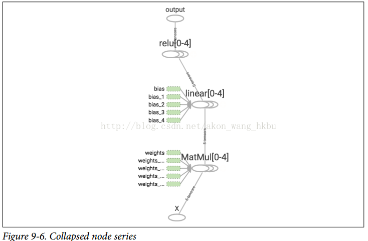
Note that when a node is created, TensorFlow checks to see if its name already exists, and if it already exists, an underscore is appended followed by an index to make the name unique.Therefore, the first ReLU contains nodes named weights, bias, z, and relu (plus more nodes with other default names, such as MatMul); the second ReLU contains nodes named weights_1, bias_1, and so on; the third ReLU contains nodes named weights_2, bias_2, and so on.TensorBoard identifies such series and folds them together to reduce clutter (as shown in Figures 9-6)
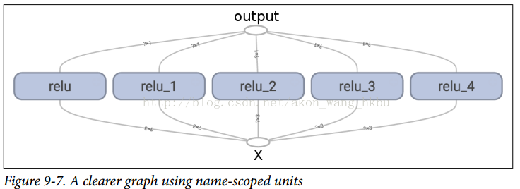
Using the name scope, you can make the graph clearer.Simply move all the contents of the relu() function into the name scope.Figures 9-7 show the results.Note that TensorFlow also provides a unique name for the name scope by appending _1, _2, and so on.
def relu(X):
    with tf.name_scope("relu"):
        w_shape = (int(X.get_shape()[1]), 1)                          # not shown in the book
        w = tf.Variable(tf.random_normal(w_shape), name="weights")    # not shown
        b = tf.Variable(0.0, name="bias")                             # not shown
        z = tf.add(tf.matmul(X, w), b, name="z")                      # not shown
        return tf.maximum(z, 0., name="max")                          # not shown
Shared variable
If you want to share a variable among the components of a graph, a simple option is to create it first and pass it as a parameter to the function that needs it.For example, suppose you want to use a shared threshold variable for all ReLUs to control the ReLU threshold (currently hard coded as 0).You can create the variable and pass it to the relu() function:
reset_graph()

def relu(X, threshold):
    with tf.name_scope("relu"):
        w_shape = (int(X.get_shape()[1]), 1)                        # not shown in the book
        w = tf.Variable(tf.random_normal(w_shape), name="weights")  # not shown
        b = tf.Variable(0.0, name="bias")                           # not shown
        z = tf.add(tf.matmul(X, w), b, name="z")                    # not shown
        return tf.maximum(z, threshold, name="max")

threshold = tf.Variable(0.0, name="threshold")
X = tf.placeholder(tf.float32, shape=(None, n_features), name="X")
relus = [relu(X, threshold) for i in range(5)]
output = tf.add_n(relus, name="output")
That's good: Now you can use the threshold variable to control the thresholds for all ReLUs.However, if you have many shared parameters, such as this one, you must always pass them as parameters, which can be painful.Many people create a Python dictionary that contains all the variables in a model and pass it to each function.Others create a class for each module (for example, a ReLU class that uses class variables to handle shared parameters).Another option is to set the shared variable as a property of the relu() function on the first call, as follows:
def relu(X):
    with tf.name_scope("relu"):
        if not hasattr(relu, "threshold"):
            relu.threshold = tf.Variable(0.0, name="threshold")
        w_shape = int(X.get_shape()[1]), 1                          # not shown in the book
        w = tf.Variable(tf.random_normal(w_shape), name="weights")  # not shown
        b = tf.Variable(0.0, name="bias")                           # not shown
        z = tf.add(tf.matmul(X, w), b, name="z")                    # not shown
        return tf.maximum(z, relu.threshold, name="max")
TensorFlow offers another option that will provide slightly cleaner and more modular code than previous solutions.The first thing to understand is that this solution is tricky, but because it's used a lot in TensorFlow, it's worth going into the details.The idea is to use the get_variable() function to create a shared variable and reuse it if it does not already exist or if it already exists.The desired behavior (creation or reuse) is controlled by the properties of the current variable_scope().For example, the following code creates a variable named relu/threshold s (as a scalar because shape = () and uses 0.0 as the initial value):
with tf.variable_scope("relu"):
    threshold = tf.get_variable("threshold", shape=(),
                                initializer=tf.constant_initializer(0.0))
Note that if a variable has been created by an earlier get_variable() call, this code will throw an exception.This behavior prevents erroneous reuse of variables.If you want to reuse variables, you need to make it clear by setting the variable scope's reuse property to True (in which case you don't have to specify a shape or initial value):
with tf.variable_scope("relu", reuse=True):
    threshold = tf.get_variable("threshold")
This code takes an existing relu/threshold variable, if none exists it will throw an exception if it is not created using get_variable().Alternatively, you can set the reuse property to true by calling reuse_variables() of scope:
with tf.variable_scope("relu") as scope:
    scope.reuse_variables()
    threshold = tf.get_variable("threshold")
Once reuse is set to True, it cannot be set to False within a block.Also, if other variable scopes are defined in them, they automatically inherit reuse = True.Finally, only variables created by get_variable() can be reused in this way.
Now you have all the parts you need to make the relu() function access the threshold variable without passing it as a parameter:
def relu(X):
    with tf.variable_scope("relu", reuse=True):
        threshold = tf.get_variable("threshold")
        w_shape = int(X.get_shape()[1]), 1                          # not shown
        w = tf.Variable(tf.random_normal(w_shape), name="weights")  # not shown
        b = tf.Variable(0.0, name="bias")                           # not shown
        z = tf.add(tf.matmul(X, w), b, name="z")                    # not shown
        return tf.maximum(z, threshold, name="max")

X = tf.placeholder(tf.float32, shape=(None, n_features), name="X")
with tf.variable_scope("relu"):
    threshold = tf.get_variable("threshold", shape=(),
                                initializer=tf.constant_initializer(0.0))
relus = [relu(X) for relu_index in range(5)]
output = tf.add_n(relus, name="output")
The code first defines the relu() function, then creates the relu/threshold variable (which will be initialized to 0.0 later as a scalar), and builds five ReLUs by calling the relu() function.The relu() function multiplies the relu/threshold variable and creates other ReLU nodes.
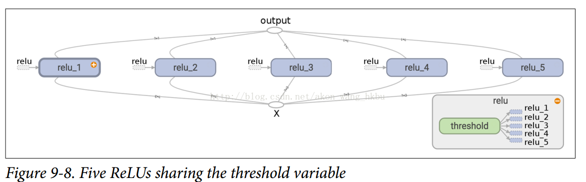
Variables created with get_variable() are always prefixed with the name of their variable_scope (for example, relu/threshold), but for all other nodes, including variables created with tf.Variable(), the variable scope behaves like a scope with a new name.In particular, if a name scope with the same name has been created, add a suffix to make the name unique.For example, all nodes created in the preceding code (except threshold variables) have names prefixed with relu_1/to relu_5/, as shown in Figures 9-8.
Unfortunately, threshold variables must be defined outside the relu() function, where the rest of the ReLU code resides.To solve this problem, the following code creates a threshold variable in the relu() function on the first call and reuses it in subsequent calls.Now, the relu() function doesn't have to worry about name scope or variable sharing: it just calls get_variable(), which creates or reuses threshold variables (it doesn't need to know what that is).The rest of the code calls relu () five times, ensuring that reuse = False is set on the first call, and for other calls, reuse = True.
def relu(X):
    threshold = tf.get_variable("threshold", shape=(),
                                initializer=tf.constant_initializer(0.0))
    w_shape = (int(X.get_shape()[1]), 1)                        # not shown in the book
    w = tf.Variable(tf.random_normal(w_shape), name="weights")  # not shown
    b = tf.Variable(0.0, name="bias")                           # not shown
    z = tf.add(tf.matmul(X, w), b, name="z")                    # not shown
    return tf.maximum(z, threshold, name="max")

X = tf.placeholder(tf.float32, shape=(None, n_features), name="X")
relus = []
for relu_index in range(5):
    with tf.variable_scope("relu", reuse=(relu_index >= 1)) as scope:
        relus.append(relu(X))
output = tf.add_n(relus, name="output")
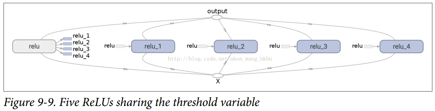
The resulting graph is slightly different from the previous one because the shared variable exists in the first ReLU (see Figures 9-9).
This concludes the introduction to TensorFlow.We will discuss more advanced topics in the following chapters, especially many operations related to deep neural networks, convolution and recursive neural networks, and how to use multithreading, queues, multiple GPU s, and how to extend TensorFlow to multiple servers.