Gray Histogram Source Code
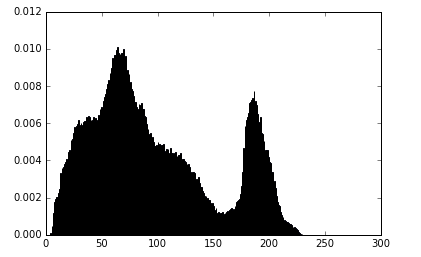
The essence of gray histogram is to count the probability of gray occurrence of each pixel in an image.
Abscissa: 0-255 ordinate probability p (0-1)
# 10-2552 probability
import cv2
import numpy as np
import matplotlib.pyplot as plt
%matplotlib inline
img = cv2.imread('image0.jpg',1)
imgInfo = img.shape
height = imgInfo[0]
width = imgInfo[1]
# Grayscale
gray = cv2.cvtColor(img,cv2.COLOR_BGR2GRAY)
# count records the probability of each gray value appearing
count = np.zeros(256,np.float)
# for loop traverses every point in the picture
for i in range(0,height):
    for j in range(0,width):
        # Get the gray value of the current picture
        pixel = gray[i,j]
        # Convert to int type
        index = int(pixel)
        # Let's take this gray scale factor, like count's 255 element, which was originally zero now + 1
        count[index] = count[index]+1
# The gray level is counted and the probability of occurrence is calculated.
for i in range(0,255):
    count[i] = count[i]/(height*width)
# Drawing Method Using Matplotlib
# Number of 0-255: 256
x = np.linspace(0,255,256)
y = count
plt.bar(x,y,0.8,alpha=1,color='b')
plt.show()
cv2.waitKey(0)
mark
Using Inline to display the color in the browser is incorrect. And delete this line is blue.
Color Histogram Source Code
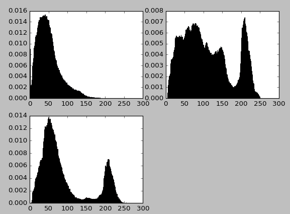
# Essence: Statistical probability of gray level occurrence for each pixel is 0-255 p
# For color histogram, three channels are counted separately.
import cv2
import numpy as np
import matplotlib.pyplot as plt
%matplotlib inline
img = cv2.imread('image0.jpg',1)
imgInfo = img.shape
height = imgInfo[0]
width = imgInfo[1]

# b-channel probability
count_b = np.zeros(256,np.float)
count_g = np.zeros(256,np.float)
count_r = np.zeros(256,np.float)

# for loop traverses every point
for i in range(0,height):
    for j in range(0,width):
        (b,g,r) = img[i,j]
        index_b = int(b)
        index_g = int(g)
        index_r = int(r)
        count_b[index_b] = count_b[index_b]+1
        count_g[index_g] = count_g[index_g]+1
        count_r[index_r] = count_r[index_r]+1

# Computing probability
for i in range(0,256):
    count_b[i] = count_b[i]/(height*width)
    count_g[i] = count_g[i]/(height*width)
    count_r[i] = count_r[i]/(height*width)

# Drawing lines, x-axis coordinates
x = np.linspace(0,255,256)
plt.figure(12)
y1 = count_b
plt.subplot(221)
plt.bar(x,y1,0.9,alpha=1,color='b')
y2 = count_g
plt.subplot(222)
plt.bar(x,y2,0.9,alpha=1,color='g')
y3 = count_r
plt.subplot(223)
plt.bar(x,y3,0.9,alpha=1,color='r')
plt.show()
cv2.waitKey(0)
mark
I don't know why the color is wrong.
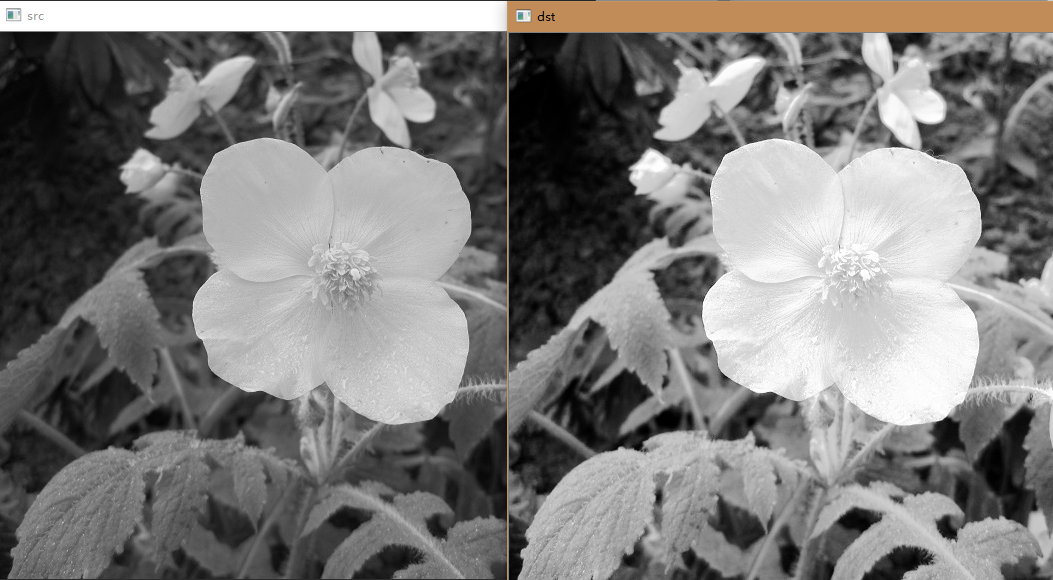
histogram equalization
# Essence of Histogram: Statistical probability of occurrence of gray level of each pixel is 0-255 p(0-1)

# Histogram equalization means:

# The concept of cumulative probability
# The occurrence probability of the first gray level is 0.2 and the cumulative probability is 0.2.
# The second gray level occurrence probability is 0.3 cumulative probability 0.5 (0.2 + 0.3)
# The third gray level occurrence probability is 0.1 cumulative probability 0.6 (0.5 + 0.1)
# 256 gray levels, each gray level will have a probability and a cumulative probability
# 100 This gray level has a cumulative probability of 0.5,255*0.5=the value of new
# You can get a mapping of 100 to a new value
# After that, all gray levels of 100 are replaced by 255*0.5.

# This process is called histogram equalization.

import cv2
import numpy as np
import matplotlib.pyplot as plt
img = cv2.imread('image0.jpg',1)


imgInfo = img.shape
height = imgInfo[0]
width = imgInfo[1]

# Grayscale
gray = cv2.cvtColor(img,cv2.COLOR_BGR2GRAY)
cv2.imshow('src',gray)
count = np.zeros(256,np.float)
for i in range(0,height):
    for j in range(0,width):
        pixel = gray[i,j]
        index = int(pixel)
        count[index] = count[index]+1
# Calculating single probability of gray level
for i in range(0,255):
    count[i] = count[i]/(height*width)

#Calculating cumulative probability
sum1 = float(0)
for i in range(0,256):
    sum1 = sum1+count[i]
    count[i] = sum1

# At this point count stores the cumulative probability corresponding to each gray level.

# print(count)
# Compute the mapping table data type to unit16
map1 = np.zeros(256,np.uint16)

for i in range(0,256):
    # Because the count value at this time is the cumulative probability, multiply 255 as the real mapping value.
    map1[i] = np.uint16(count[i]*255)
# Completion mapping
for i in range(0,height):
    for j in range(0,width):
        pixel = gray[i,j]
        # The subscript of the mapping table is obtained from the current gray value to the mapping value.
        gray[i,j] = map1[pixel]
cv2.imshow('dst',gray)
cv2.waitKey(0)
mark
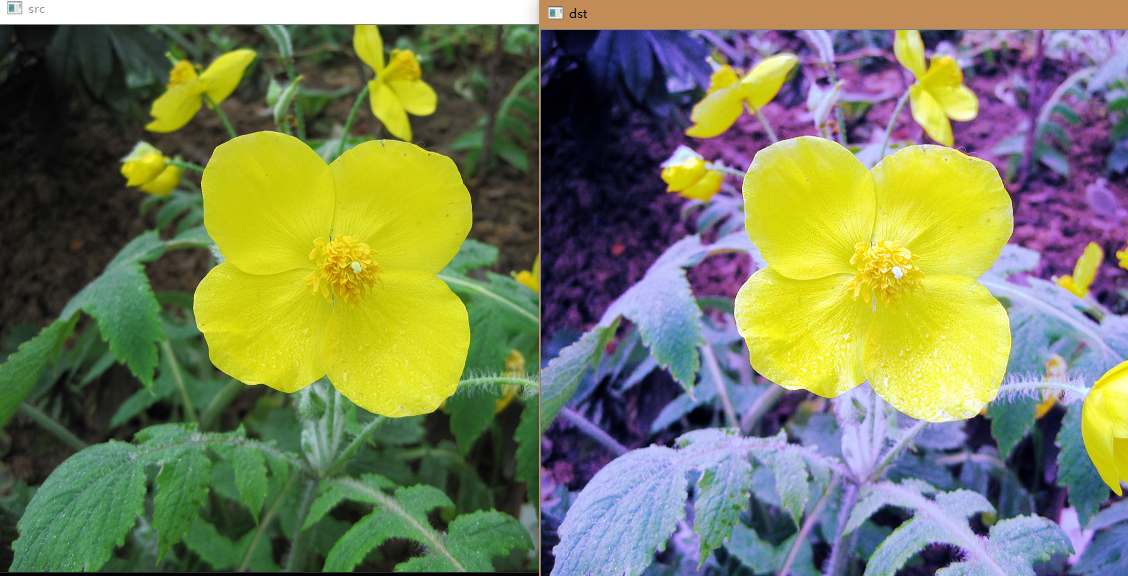
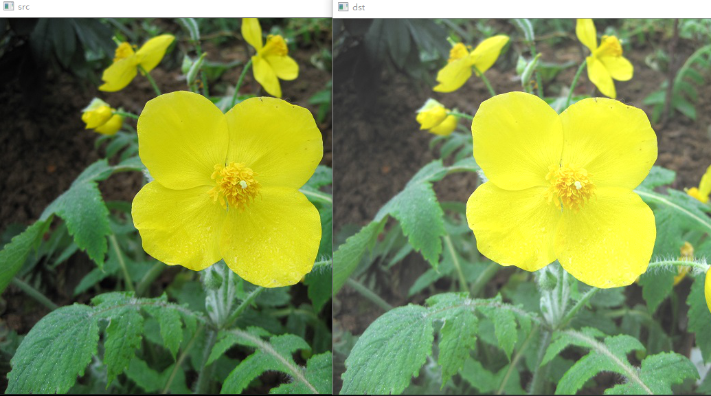
Color histogram equalization
# Essence: Statistical probability of gray level occurrence for each pixel is 0-255 p
# Cumulative probability
# 1 0.2  0.2
# 2 0.3  0.5
# 3 0.1  0.6
# 256
# 100 0.5 255*0.5 = new
# 1 Statistical probability of each color 2 Cumulative probability 1 30-255 255*p
# 4 pixel
import cv2
import numpy as np
import matplotlib.pyplot as plt
img = cv2.imread('image0.jpg',1)
cv2.imshow('src',img)

imgInfo = img.shape
height = imgInfo[0]
width = imgInfo[1]

# Three count s, describing the probability of color occurrence, respectively
count_b = np.zeros(256,np.float)
count_g = np.zeros(256,np.float)
count_r = np.zeros(256,np.float)
# Get the number of color values corresponding to all the pixels
for i in range(0,height):
    for j in range(0,width):
        (b,g,r) = img[i,j]
        index_b = int(b)
        index_g = int(g)
        index_r = int(r)
        count_b[index_b] = count_b[index_b]+1
        count_g[index_g] = count_g[index_g]+1
        count_r[index_r] = count_r[index_r]+1
# Calculate the probability of each occurrence
for i in range(0,255):
    count_b[i] = count_b[i]/(height*width)
    count_g[i] = count_g[i]/(height*width)
    count_r[i] = count_r[i]/(height*width)

# Calculating cumulative probability
sum_b = float(0)
sum_g = float(0)
sum_r = float(0)
for i in range(0,256):
    sum_b = sum_b+count_b[i]
    sum_g = sum_g+count_g[i]
    sum_r = sum_r+count_r[i]
    count_b[i] = sum_b
    count_g[i] = sum_g
    count_r[i] = sum_r

#print(count)
# Computing three mapping tables
map_b = np.zeros(256,np.uint16)
map_g = np.zeros(256,np.uint16)
map_r = np.zeros(256,np.uint16)

# Create three mapping tables
for i in range(0,256):
    map_b[i] = np.uint16(count_b[i]*255)
    map_g[i] = np.uint16(count_g[i]*255)
    map_r[i] = np.uint16(count_r[i]*255)
# mapping
# Final data
dst = np.zeros((height,width,3),np.uint8)

# Read each point and map it
for i in range(0,height):
    for j in range(0,width):
        (b,g,r) = img[i,j]
        b = map_b[b]
        g = map_g[g]
        r = map_r[r]
        # Target Picture Data Filling
        dst[i,j] = (b,g,r)
cv2.imshow('dst',dst)
cv2.waitKey(0)
mark
Brightness enhancement
Formula:
p = p + 40
Brightness enhancement is accomplished after simple addition.
# p = p + 40
import cv2
import numpy as np
img = cv2.imread('image0.jpg',1)
imgInfo = img.shape
height = imgInfo[0]
width = imgInfo[1]
cv2.imshow('src',img)

# The final image data we generated
dst = np.zeros((height,width,3),np.uint8)
# Traverse through each point in the picture
for i in range(0,height):
    for j in range(0,width):
        # Take out three channels at each point
        (b,g,r) = img[i,j]
        bb = int(b)+40
        gg = int(g)+40
        rr = int(r)+40
        # Judgment does not go beyond boundaries
        if bb>255:
            bb = 255
        if gg>255:
            gg = 255
        if rr>255:
            rr = 255
        # Data Fill in Target Picture
        dst[i,j] = (bb,gg,rr)
cv2.imshow('dst',dst)
cv2.waitKey(0)
mark
The brightness of the picture did increase, but it seemed to be covered with a white mask.