Label
PostgreSQL, HTAP, OLTP, OLAP, Scenario and Performance Testing
background
PostgreSQL is a database with a long history, which can be traced back to 1973. It was first awarded by the 2014 Computer Turing Prize winner and the originator of relational database. Michael_Stonebraker PostgreSQL has similar functions, performance, architecture and stability as Oracle.
The PostgreSQL community has many contributors, from all walks of life around the world. Over the years, PostgreSQL releases a large version every year, known for its enduring vitality and stability.
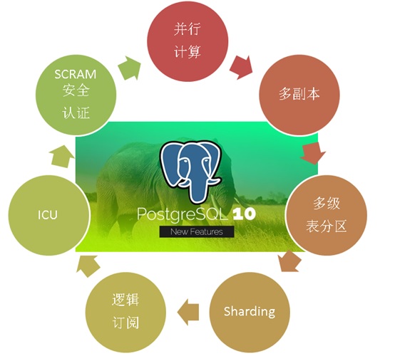
In October 2017, PostgreSQL released version 10, which carries many amazing features. The goal is to meet the requirements of mixed HTAP scenarios of OLAP and OLTP:
PostgreSQL 10 features, the most popular HTAP database for developers
1. Multi-core Parallel Enhancement
2. fdw aggregation push-down
3. Logical Subscription
4, zoning
5. Multi-copies at the financial level
6. json, jsonb full-text retrieval
7. There are also some features of plug-in form, such as vector computing, JIT, SQL graph computing, SQL stream computing, distributed parallel computing, time series processing, gene sequencing, chemical analysis, image analysis, etc.
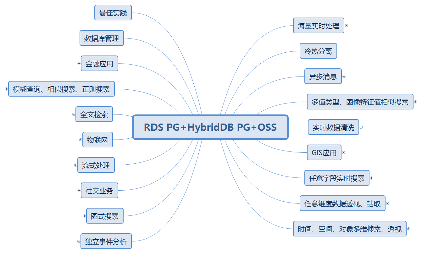
PostgreSQL can be seen in various application scenarios:
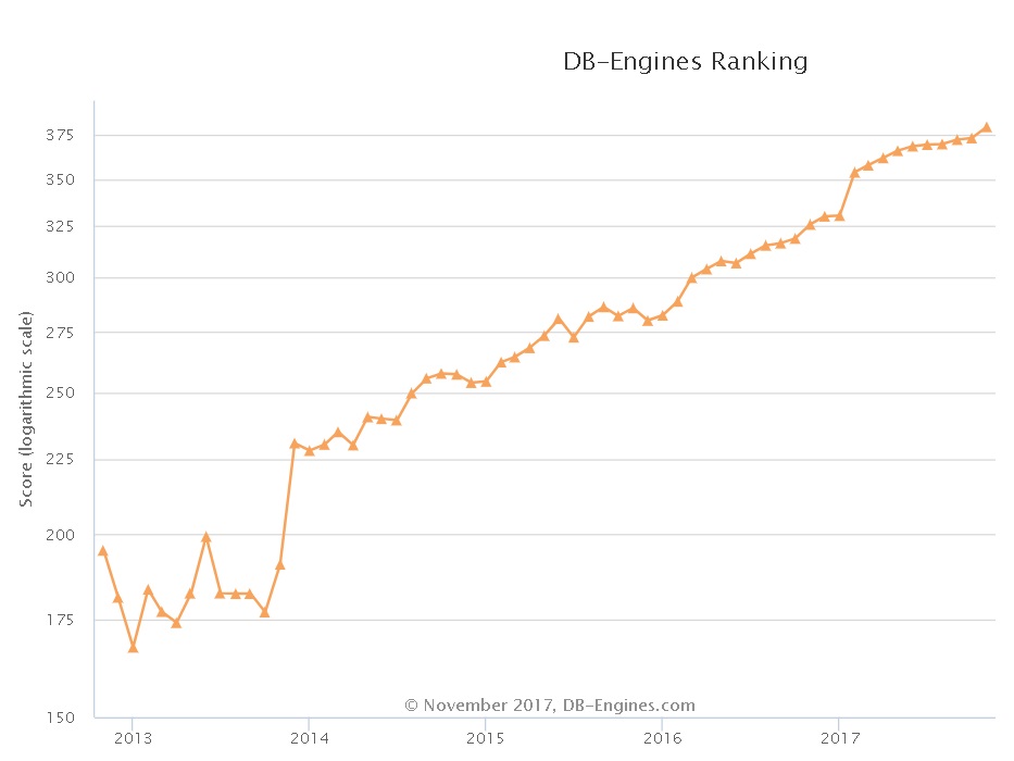
PostgreSQL has developed very rapidly in recent years. From the database scoring trend of dbranking, a well-known database evaluation website, we can see the upward trend of PostgreSQL:
From the annual community meetings held in PostgreSQL China, we can see the same trend. More and more companies are participating, more and more companies are sharing, and more and more subjects are shared. They span traditional enterprises, Internet, medical, financial, state-owned enterprises, logistics, e-commerce, social networking, vehicle networking, sharing XX, cloud, game, public transport, aviation, railway, military, training. Training, consulting services, etc.
The next series of articles will introduce various application scenarios and corresponding performance indicators of PostgreSQL.
Environmental Science
Reference to Environmental Deployment Method:
Aliyun ECS: 56 core, 224G, 1.5TB*2 SSD cloud disk.
Operating System: CentOS 7.4 x64
Database version: PostgreSQL 10
PS: The CPU and IO performance of ECS is discounted by physical opportunity, and can be estimated by one-fold performance decline. Running physical mainframe can be estimated by multiplying the performance tested here by 2.
Scenario-Sorting, Indexing (OLTP+OLAP)
1, background
1. In OLTP, sorting is usually the sorting of small data sets.
2. In OLAP, it is usually necessary to sort large result sets and select TOP.
3. The speed of sorting also directly affects the speed of index building. (Note that PostgreSQL supports CONCURRENTLY to build indexes without blocking DML.)
4. In OLAP, there are some simple and efficient methods to extract TOP: estimation, HLL, sampling, statistical information, etc.
<PostgreSQL hll (HyperLogLog) extension for "State of The Art Cardinality Estimation Algorithm" - 1>
<PostgreSQL hll (HyperLogLog) extension for "State of The Art Cardinality Estimation Algorithm" - 2>
<PostgreSQL hll (HyperLogLog) extension for "State of The Art Cardinality Estimation Algorithm" - 3>
Quick Line Estimation Using explain Plan Rows
2, design
1. Sort small data, 10,000 pieces of data.
2. Sorting large amount of data and 100 million pieces of data.
3. The efficiency of index creation with large amount of data is 100 million pieces of data.
4. Big data valuation TOP N, 100 million data.
5. Big data, composite index, seek the ID of TOP c2 of any GROUP C 1, 100 million data.
3. Preparing test sheets
create table t_small (id int);

create table t_large (id int);

create table t_estimate (id int);

create table t_idx_test (id int, c1 int, c2 int);
4. Preparing test functions (optional)
5. Preparing test data
1. Sort small data, 10,000 pieces of data.
insert into t_small select generate_series(1,10000);
2. Sorting large amount of data and 100 million pieces of data.
insert into t_large select generate_series(1,100000000);
4. Big data valuation TOP N, 100 million data.
vi test.sql

\set id random_gaussian(1, 1000000, 2.5)
insert into t_estimate values (:id);
pgbench -M prepared -n -r -P 5 -f ./test.sql -c 50 -j 50 -t 2000000
analyze t_estimate;
5. Big data, composite index, seek the ID of TOP c2 of any GROUP C 1, 100 million data.
insert into t_idx_test select id, random()*1000, random()*900000 from generate_series(1,100000000) t(id);
create index idx_t_idx_test on t_idx_test (c1,c2);
6. Preparing test scripts
vi test.sql

\set c1 random(1,1000)
select id from t_idx_test where c1=:c1 order by c2 desc limit 1;
Pressure measurement
CONNECTS=112
TIMES=300
export PGHOST=$PGDATA
export PGPORT=1999
export PGUSER=postgres
export PGPASSWORD=postgres
export PGDATABASE=postgres

pgbench -M prepared -n -r -f ./test.sql -P 5 -c $CONNECTS -j $CONNECTS -T $TIMES
7, test
1. Sorting of Small Data Quantity
postgres=# explain (analyze,verbose,timing,costs,buffers) select * from t_small order by id desc limit 1;
                                                          QUERY PLAN
------------------------------------------------------------------------------------------------------------------------------
 Limit  (cost=195.00..195.00 rows=1 width=4) (actual time=2.580..2.581 rows=1 loops=1)
   Output: id
   Buffers: shared hit=45
   ->  Sort  (cost=195.00..220.00 rows=10000 width=4) (actual time=2.580..2.580 rows=1 loops=1)
         Output: id
         Sort Key: t_small.id DESC
         Sort Method: top-N heapsort  Memory: 25kB
         Buffers: shared hit=45
         ->  Seq Scan on public.t_small  (cost=0.00..145.00 rows=10000 width=4) (actual time=0.006..1.184 rows=10000 loops=1)
               Output: id
               Buffers: shared hit=45
 Planning time: 0.027 ms
 Execution time: 2.591 ms
(13 rows)
2. Sorting of Large Data Volume
alter table t_large set (parallel_workers =32);
set parallel_setup_cost =0;
set parallel_tuple_cost =0;
set max_parallel_workers_per_gather =32;
set work_mem ='1GB';
explain select * from t_large order by id desc limit 1;

postgres=# explain select * from t_large order by id desc limit 1;
                                         QUERY PLAN
---------------------------------------------------------------------------------------------
 Limit  (cost=810844.97..810845.00 rows=1 width=4)
   ->  Gather Merge  (cost=810844.97..3590855.42 rows=100000032 width=4)
         Workers Planned: 32
         ->  Sort  (cost=810844.14..818656.64 rows=3125001 width=4)
               Sort Key: id DESC
               ->  Parallel Seq Scan on t_large  (cost=0.00..473728.01 rows=3125001 width=4)
(6 rows)

postgres=# select * from t_large order by id desc limit 1;
    id
-----------
 100000000
(1 row)
Time: 1482.964 ms (00:01.483)
3. Index Creation Efficiency for Large Data Volume
postgres=# create index idx_t_large_id on t_large(id);
CREATE INDEX
Time: 37937.482 ms (00:37.937)
4. TOP N of Big Data Valuation
postgres=# select most_common_vals, most_common_freqs from pg_stats where tablename='t_estimate';
-[ RECORD 1 ]-----+-------------------------------------------------------------------------------------------------------------------------------------------------------------------------------------------------------------------------------------------------------------------------------------------------------------------------------------------------------------------------------------------------------------------------------------------------------------------------------------------------------------------------------------------------------------------------------------------------------------------------------------------------------------------------------------------------------------------------------------------------------------------------------------------------------------------------------------------------------------------------------------------------------------------------------------------------------------------------------------------------------------------------------------------------------------------------------------------------------------------------------------------------------------------------------------------
most_common_vals  | {354316,354445,404899,431899,451975,525707,545934,552219,631936,654703,686785,52824,97919,100231,134912,137688,158267,161541,171349,182376,182892,186086,192265,196224,197934,206937,207098,208325,213459,218788,218939,225221,226377,238291,239857,245513,245868,250632,250836,251535,251972,254658,254998,255236,256667,259600,260215,263041,266027,268086,271091,271490,271520,272019,272459,282086,286285,287848,288015,288233,288310,288344,288605,289181,289901,291581,296327,301385,301631,304765,304923,306094,306309,307188,312000,313190,313449,315581,317808,320374,320769,322517,322889,323389,326463,326738,330239,331553,334323,335451,335588,337521,338605,342766,344188,344662,344730,345081,345096,346053}
most_common_freqs | {0.0001,0.0001,0.0001,0.0001,0.0001,0.0001,0.0001,0.0001,0.0001,0.0001,0.0001,6.66667e-05,6.66667e-05,6.66667e-05,6.66667e-05,6.66667e-05,6.66667e-05,6.66667e-05,6.66667e-05,6.66667e-05,6.66667e-05,6.66667e-05,6.66667e-05,6.66667e-05,6.66667e-05,6.66667e-05,6.66667e-05,6.66667e-05,6.66667e-05,6.66667e-05,6.66667e-05,6.66667e-05,6.66667e-05,6.66667e-05,6.66667e-05,6.66667e-05,6.66667e-05,6.66667e-05,6.66667e-05,6.66667e-05,6.66667e-05,6.66667e-05,6.66667e-05,6.66667e-05,6.66667e-05,6.66667e-05,6.66667e-05,6.66667e-05,6.66667e-05,6.66667e-05,6.66667e-05,6.66667e-05,6.66667e-05,6.66667e-05,6.66667e-05,6.66667e-05,6.66667e-05,6.66667e-05,6.66667e-05,6.66667e-05,6.66667e-05,6.66667e-05,6.66667e-05,6.66667e-05,6.66667e-05,6.66667e-05,6.66667e-05,6.66667e-05,6.66667e-05,6.66667e-05,6.66667e-05,6.66667e-05,6.66667e-05,6.66667e-05,6.66667e-05,6.66667e-05,6.66667e-05,6.66667e-05,6.66667e-05,6.66667e-05,6.66667e-05,6.66667e-05,6.66667e-05,6.66667e-05,6.66667e-05,6.66667e-05,6.66667e-05,6.66667e-05,6.66667e-05,6.66667e-05,6.66667e-05,6.66667e-05,6.66667e-05,6.66667e-05,6.66667e-05,6.66667e-05,6.66667e-05,6.66667e-05,6.66667e-05,6.66667e-05}

Time: 1.274 ms
5. Big data, composite index, seek the ID of TOP c2 of any GROUP C 1, 100 million data.
transaction type: ./test.sql
scaling factor: 1
query mode: prepared
number of clients: 112
number of threads: 112
duration: 300 s
number of transactions actually processed: 203376551
latency average = 0.165 ms
latency stddev = 0.324 ms
tps = 677702.381595 (including connections establishing)
tps = 677897.901150 (excluding connections establishing)
script statistics:
 - statement latencies in milliseconds:
         0.002  \set c1 random(1,1000)
         0.168  select id from t_idx_test where c1=:c1 order by c2 desc limit 1;
TPS: 677897
5. Big data, composite index, seek the ID of TOP c2 of any GROUP C 1, 100 million data. TPS:677897
Average response time: 0.165 milliseconds
1. Sorting small amount of data, 10,000 pieces of data, Sorting takes 2.6 milliseconds.
2. Sorting large amount of data, 100 million pieces of data, and sorting takes 1.48 seconds.
3. It takes 37.9 seconds to create index with 100 million pieces of data.
4. Big data estimates TOP N, 1 data, estimates TOP N, takes 1.27 milliseconds.
5. Big data, composite index, seek the ID of TOP c2 of any GROUP C 1, 100 million data. Average response time: 0.165 milliseconds.
Reference resources
PostgreSQL, Greenplum Application Case Book "Tathagata Palm" - Catalogue
"Database Selection - Elephant Eighteen Touches - To Architects and Developers"
PostgreSQL uses pgbench to test sysbench related case s


