This tutorial is open source: GitHub Welcome, star

1, Normal estimation

1. Parameter description

Since almost all classes in PCL inherit from the basic pcl::PCLBase class, the pcl::Feature class accepts input data in two different ways:

1. A complete point cloud data set is forced through setinputcloud (pointcloudconstptr &)

   Any feature estimation class will attempt to estimate the features of each point in a given input cloud.

2. Subset of point cloud dataset, given by setinputcloud (pointcloudconstptr &) and setindexes (indicesconstptr &) - Optional

   Any feature estimation class will attempt to estimate the feature of each point in a given input cloud that has an index in a given index list. By default, if a set of indexes is not given, all points in the cloud are considered.

In addition, you can specify the set of point neighbors to use through an additional call * * setsearksurface (pointcloudconstptr &) * * to. This call is optional. When no search face is given, the input point cloud dataset is used by default.

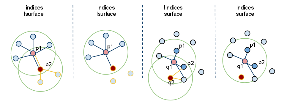
Because * * setInputCloud() * is always needed, we can create up to four combinations with < setInputCloud(), setindexes(), setsearchsurface() > *. Suppose we have two point clouds, P={p_1, p_2,... p_n} and Q={q_1, q_2,..., q_n}. The following figure shows all four cases:

• Setindexes() = false, setsearchsurface() = false - this is undoubtedly the most common case in PCL, where the user just enters a single PointCloud dataset and expects to estimate a feature at all points in the cloud.

  Since we do not want to maintain different implementation copies depending on whether a set of indexes and / or search surfaces are given, PCL will create a set of internal indexes (as std::vector) to basically point to the entire dataset (index = 1... N, where n is the number of points in the cloud) whenever index = false.

  In the figure above, this corresponds to the leftmost case. First, we estimate p_1's nearest neighbor, then P_ The nearest neighbor of 2, and so on, until we use up all points in P.

• Setindexes() = true, setsearchsurface() = false - as mentioned earlier, the feature estimation method will only calculate the features of points indexed in a given index direction;

  In the figure above, this corresponds to the second case. Here, we assume P_ The index of 2 is not part of a given index vector, so neighbors or features are not estimated in p2.

• Setindexes() = false, setSearchSurface() = true - as in the first case, the characteristics of all points given as input will be estimated, but the underlying adjacent surface given in setSearchSurface() will be used to obtain the nearest neighbor of the input, not the input cloud itself;

  In the figure above, this corresponds to the third case. If Q={q_1, q_2} is another cloud given as input, different from P, and P is the search surface of Q, then Q_ 1 and Q_ The neighbor of 2 will be calculated from P.

• Setindexes() = true, setSearchSurface() = true - this is probably the most rare case where both indexes and search surfaces are given. In this case, the search surface information given in setSearchSurface() will be used to estimate features for only a subset of < input, indices > pairs.

  Finally, in the figure above, this corresponds to the last (rightmost) case. Here, we assume Q_ The index of 2 is not part of the index vector given for Q, so neighbors or features are not estimated at q2.

The most useful example when * * setSearchSurface() * * should be used is when we have a very dense input data set, but we don't want to estimate the characteristics of all points in it, but use PCL instead_ Some key points found by the method in the keys = or in the down sampling version of the cloud (for example, obtained using the pcl::VoxelGrid filter). In this case, we pass down sampling / key input through setInputCloud() and pass the original data as setSearchSurface().

2. Examples

Once the input is determined, the adjacent points of the query point can be used to estimate the local feature representation, which means capturing the geometry of the underlying sampling surface around the query point. An important problem in describing surface geometry is to infer its direction in the coordinate system, that is, to estimate its normal. Surface normals are important properties of surfaces and are widely used in many areas, such as computer graphics applications, to apply the correct light sources that generate shadows and other visual effects (for more information, see)[ RusuDissertation]).
Code see 01_3DFeaturesWork.py

• Estimates a set of surface normals for all points in the input dataset

# Estimate normal
# All points in the input dataset estimate a set of surface normals
ne = pcl.features.NormalEstimation.PointXYZ_Normal()
ne.setInputCloud(cloud)
tree = pcl.search.KdTree.PointXYZ()
ne.setSearchMethod(tree)

cloud_normals = pcl.PointCloud.Normal()
ne.setRadiusSearch(0.003)
ne.compute(cloud_normals)
print(cloud_normals.size())

• Estimates a set of surface normals for a subset of points in the input dataset.

ne = pcl.features.NormalEstimation.PointXYZ_Normal()
ne.setInputCloud(cloud)
tree = pcl.search.KdTree.PointXYZ()
ne.setSearchMethod(tree)
ind = pcl.PointIndices()
[ind.indices.append(i) for i in range(0, cloud.size() // 2)]
ne.setIndices(ind)
cloud_normals = pcl.PointCloud.Normal()
ne.setRadiusSearch(0.003)
ne.compute(cloud_normals)
print(cloud_normals.size())

• One set of surface normals is estimated for all points in the input dataset, but their nearest neighbors are estimated using another dataset

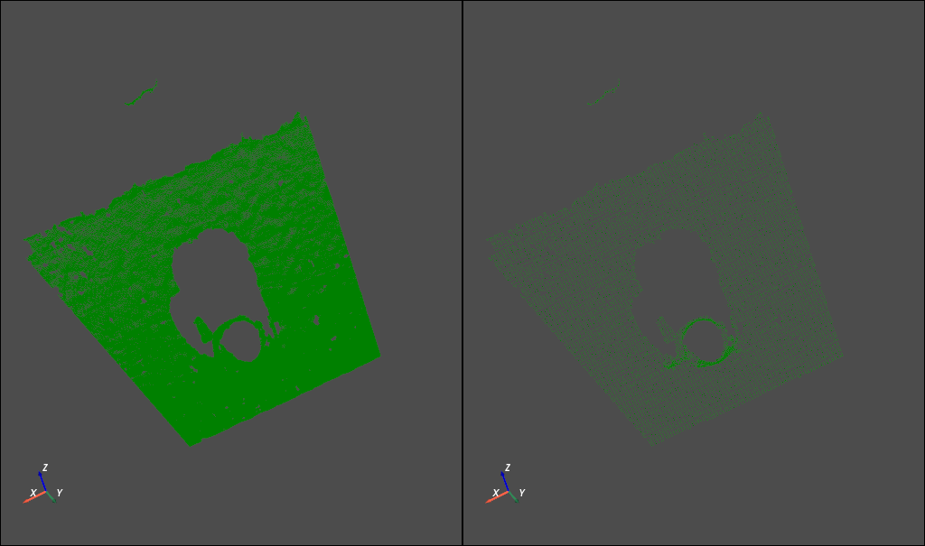
  Here, we use the down sampling point cloud of the point cloud as the input point cloud and the origin cloud as the SearchSurface.

ne = pcl.features.NormalEstimation.PointXYZ_Normal()
cloud_downsampled = pcl.PointCloud.PointXYZ()  # There are many methods to obtain a downsampled point cloud. voxelized method is used here
vox = pcl.filters.VoxelGrid.PointXYZ()
vox.setInputCloud(cloud)
vox.setLeafSize(0.005, 0.005, 0.005)
vox.filter(cloud_downsampled)
ne.setInputCloud(cloud_downsampled)
ne.setSearchSurface(cloud)
tree = pcl.search.KdTree.PointXYZ()
ne.setSearchMethod(tree)
cloud_normals = pcl.PointCloud.Normal()
ne.setRadiusSearch(0.003)
ne.compute(cloud_normals)
print(cloud_normals.size())

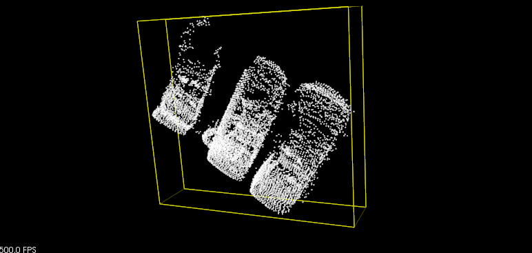
The following figure shows the original electric cloud and the down sampling point cloud respectively.

For details, please refer to how-3d-features-work , this document will not be repeated.

2, Normal estimation using integral images

In this tutorial, we will learn how to calculate the normals of an organized point cloud using an integral image.

1. Code

see 03_normal_estimation_using_integral_images.py

# Load point cloud
cloud = pcl.PointCloud.PointXYZ()
reader = pcl.io.PCDReader()
reader.read("../../data/table_scene_mug_stereo_textured.pcd", cloud)
# Estimate normal
normals = pcl.PointCloud.Normal()
ne = pcl.features.IntegralImageNormalEstimation.PointXYZ_Normal()
ne.setNormalEstimationMethod(ne.AVERAGE_3D_GRADIENT)
ne.setMaxDepthChangeFactor(0.02)
ne.setNormalSmoothingSize(10.0)
ne.setInputCloud(cloud)
ne.compute(normals)

# # visualization
# viewer = pcl.visualization.PCLVisualizer("viewer")
# viewer.setBackgroundColor(0.0, 0.0, 0.0)
# viewer.addPointCloud(cloud, "sample cloud")  # Show point cloud
# # viewer.addPointCloudNormals(cloud, normals)  # Show point clouds and normals. This function bug has not been fixed~
#
# while not viewer.wasStopped():
#     viewer.spinOnce(10)

# Visualization using pyvista
p = pv.Plotter()
cloud = pv.wrap(cloud.xyz)
p.add_mesh(cloud, point_size=1, color='g')
p.camera_position = 'iso'
p.enable_parallel_projection()
p.show_axes()
p.show()

The following error was encountered while visualizing normals:

In..\Rendering\Core\vtkActor.cxx, line 43. Error: no override found for vtkactor

After checking the official Issue of pclpy, I found that someone mentioned this Issue, and this bug has not been fixed

issue:https://github.com/davidcaron/pclpy/issues/58

It seems that pclpy has a lot of bug s in visualization (at present, it has been found that mesh and point cloud with normals cannot be visualized). In python, pyvista can be used to replace the visualization function. In fact, the author may also be aware of this problem and remove the visualization module in the latest pclpy v1.12.0.

2. Description

Here only pick a few important lines of code.

# Estimate normal
normals = pcl.PointCloud.Normal()
ne = pcl.features.IntegralImageNormalEstimation.PointXYZ_Normal()
ne.setNormalEstimationMethod(ne.AVERAGE_3D_GRADIENT)
ne.setMaxDepthChangeFactor(0.02)
ne.setNormalSmoothingSize(10.0)
ne.setInputCloud(cloud)
ne.compute(normals)

The following general estimation methods can be used:

enum NormalEstimationMethod
{
  COVARIANCE_MATRIX,
  AVERAGE_3D_GRADIENT,
  AVERAGE_DEPTH_CHANGE
};

The COVARIANCE_MATRIX mode creates 9 integral images to calculate the normals of specific points according to the covariance matrix of their local neighborhood. The AVERAGE_3D_GRADIENT mode creates 6 integral images to calculate the smooth versions of horizontal and vertical 3D gradients, and uses the cross product between the two gradients to calculate the normals. The AVERAGE_DEPTH_CHANGE mode creates only a single integral image and calculates the normals according to the average depth Calculate normals for degree changes.

reference resources: Normal Estimation Using Integral Images

3, Point feature histogram (PFH)

For the theoretical part, please refer to RusuDissertation . it will not be repeated here.

1. Code

Point feature histogram as pcl_features Part of the library is implemented in PCL.

The default PFH implementation uses five sub bins (for example, each of the four eigenvalues will use so many sub bins in its value range) and does not include the distance (as described above - although the user can call the computePairFeatures method to obtain the distance if necessary), which generates a 125 byte 5 3 5^3 53 array of floating point values (). These are stored in the PCL:: pfhsignature 125 point type.

The following code snippet will estimate a set of PFH characteristics for all points in the input dataset.
see 05_PHF_descriptors.py

import pclpy
from pclpy import pcl
import numpy as np
import sys

if __name__ == '__main__':
    # Generate point cloud data
    # Load point cloud
    cloud = pcl.PointCloud.PointXYZ()
    reader = pcl.io.PCDReader()
    reader.read("../../data/bunny.pcd", cloud)
    print(cloud.size())
    # Construct normal estimation class
    ne = pcl.features.NormalEstimation.PointXYZ_Normal()
    ne.setInputCloud(cloud)

    tree = pcl.search.KdTree.PointXYZ()
    ne.setSearchMethod(tree)

    normals = pcl.PointCloud.Normal()
    ne.setRadiusSearch(0.03)
    # Calculate normals
    ne.compute(normals)
    print(normals.size())

    # Construct PFH estimation class and pass cloud and normals in
    pfh = pcl.features.PFHEstimation.PointXYZ_Normal_PFHSignature125()
    pfh.setInputCloud(cloud)
    pfh.setInputNormals(normals)
    # Or, if the cloud is of PointNormal type, execute pfh.setInputNormals(cloud);

    # Construct a kd tree
    # Its contents will be filled into the object according to the given input point cloud (because no other search surface is given).
    tree = pcl.search.KdTree.PointXYZ()
    pfh.setSearchMethod(tree)

    # output
    pfhs = pcl.PointCloud.PFHSignature125()

    # Use neighbor points within a 5cmm sphere
    # Note: the radius used here must be greater than the radius used to estimate the surface normal!!
    pfh.setRadiusSearch(0.05)

    # Calculation characteristics
    pfh.compute(pfhs)

    print(pfhs.size())  # pfhs and cloud size should be the same

The actual calculation call from the pfestimation class does not perform any operation internally, but it does the following:

for each point p in cloud P
  1. get the nearest neighbors of p
  2. for each pair of neighbors, compute the three angular values
  3. bin all the results in an output histogram

To calculate a single PFH representation from the k-Neighborhood, the PCL can use:

computePointPFHSignature (const pcl::PointCloud<PointInT> &cloud,
                          const pcl::PointCloud<PointNT> &normals,
                          const std::vector<int> &indices,
                          int nr_split,
                          Eigen::VectorXf &pfh_histogram);

However, pclpy has not yet implemented this function.

For efficiency reasons, the calculation method in PFHEstimation does not check whether the normal contains NaN or infinite values. Passing these values to * * compute() will result in undefined output. It is recommended to check normals at least when designing processing chains or setting parameters. This can be done by inserting the following code before calling compute() *:

for i in range(normals.size()):
 if not pcl.common.isFinite(normals.at(i)):
     print('normals[%d] is not finite\n', i)

In the production code, the preprocessing steps and parameters should be set so that the normals are limited, otherwise an error will be caused.

After testing, pclpy's isfinish() function doesn't seem to support pcl.PointCloud.Normal(). emmmmm, pclpy still has a lot of bug s

reference resources: https://pcl.readthedocs.io/projects/tutorials/en/latest/pfh_estimation.html#pfh-estimation

4, Fast point feature histogram (FPFH) descriptor

For the theoretical part, please refer to: RusuDissertation , which will not be repeated here.

1. Difference between PFH and FPFH

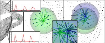
The main differences between PFH and FPFH formulations are summarized as follows:

1. p q p_q pq# as can be seen from the figure, FPFH does not have all neighbors fully interconnected, so it lacks some value pairs that may help to capture the geometry around the query point;
2. PFH models the precisely determined surface around the query point, while FPFH includes additional point pairs outside the r-radius sphere (although up to 2r away);
3. Due to the reweighting scheme, FPFH combines SPFH values and recaptures some point adjacent value pairs;
4. The overall complexity of FPFH is greatly reduced, which makes it possible to use it in real-time applications;
5. The result histogram is simplified by decorrelation value, that is, simply create d separate feature histograms, one for each feature dimension, and connect them together (see the figure below).

2. Code

The default FPFH implementation uses 11 bin subdivision (for example, each of the four eigenvalues will use so many bins from its value range) and decorrelation scheme (see above: feature histograms are calculated and combined separately), and the result is a 33 byte floating-point value array. These are stored in the pcl::FPFHSignature33 point type.

The following code snippet will estimate a set of FPFH features for all points in the input dataset.
see 06_FPFH_descriptors.py

import pclpy
from pclpy import pcl
import numpy as np
import sys

if __name__ == '__main__':
    # Generate point cloud data
    # Load point cloud
    cloud = pcl.PointCloud.PointXYZ()
    reader = pcl.io.PCDReader()
    reader.read("../../data/bunny.pcd", cloud)
    print(cloud.size())
    # Construct normal estimation class
    ne = pcl.features.NormalEstimation.PointXYZ_Normal()
    ne.setInputCloud(cloud)

    tree = pcl.search.KdTree.PointXYZ()
    ne.setSearchMethod(tree)

    normals = pcl.PointCloud.Normal()
    ne.setRadiusSearch(0.03)
    # Calculate normals
    ne.compute(normals)
    print(normals.size())
    
    # Construct FPFH estimation class and pass cloud and normals in
    fpfh = pcl.features.FPFHEstimation.PointXYZ_Normal_FPFHSignature33()
    fpfh.setInputCloud(cloud)
    fpfh.setInputNormals(normals)
    # Or, if the cloud is of PointNormal type, execute fpfh.setInputNormals(cloud);

    # Construct a kd tree
    # Its contents will be filled into the object according to the given input point cloud (because no other search surface is given).
    tree = pcl.search.KdTree.PointXYZ()
    fpfh.setSearchMethod(tree)

    # output
    pfhs = pcl.PointCloud.FPFHSignature33()

    # Use neighbor points within a 5cmm sphere
    # Note: the radius used here must be greater than the radius used to estimate the surface normal!!
    fpfh.setRadiusSearch(0.05)

    # Calculation characteristics
    fpfh.compute(pfhs)
    print(pfhs.size())  # pfhs and cloud size should be the same

The actual calculation call from the FPFHEstimation class does not perform any operation internally, but does the following:

for each point p in cloud P
  1. pass 1:
     1. get the nearest neighbors of :math:`p`
     2. for each pair of :math:`p, p_i` (where :math:`p_i` is a neighbor of :math:`p`, compute the three angular values
     3. bin all the results in an output SPFH histogram
  2. pass 2:
     1. get the nearest neighbors of :math:`p`
     3. use each SPFH of :math:`p` with a weighting scheme to assemble the FPFH of :math:`p`:

Similarly, for efficiency reasons, the calculation method in FPFHEstimation does not check whether the normal contains NaN or infinite values. Passing these values to * * compute() will result in undefined output. It is recommended to check normals at least when designing processing chains or setting parameters. This can be done by inserting the following code before calling compute() *:

for i in range(normals.size()):
 if not pcl.common.isFinite(normals.at(i)):
     print('normals[%d] is not finite\n', i)

In the production code, the preprocessing steps and parameters should be set so that the normals are limited, otherwise an error will be caused.

After testing, pclpy's isfinish() function doesn't seem to support pcl.PointCloud.Normal(). emmmmm, pclpy still has a lot of bug s

5, Estimate the VFH characteristics of a set of points

For the theoretical part, see: Use VFH descriptor And / or[ VFH]Cluster recognition and 6DOF attitude estimation It will not be repeated here.

1. Code

Viewpoint feature histogram as pcl_features Part of the library is implemented in PCL.

The default VFH implementation uses 45 sub box subdivisions for each of the three extended FPFH values, plus another 45 sub box subdivisions of the distance between each point and the centroid and 128 sub box subdivisions of the viewpoint component, resulting in a 308 byte floating-point array value. They are stored in PCL:: vfhsignature 308 point type.

The main difference between PFH/FPFH descriptor and VFH is that for a given point cloud dataset, only a single VFH descriptor will be estimated, and the generated PFH/FPFH data will have the same number of entries as the number of points.

The following code snippet will estimate a set of VFH characteristics for all points in the input dataset.

see 07_VFH_descriptors.py

cloud = pcl.PointCloud.PointXYZ()
reader = pcl.io.PCDReader()
reader.read("../../data/bunny.pcd", cloud)
print(cloud.size())
# Construct normal estimation class
ne = pcl.features.NormalEstimation.PointXYZ_Normal()
ne.setInputCloud(cloud)

tree = pcl.search.KdTree.PointXYZ()
ne.setSearchMethod(tree)

normals = pcl.PointCloud.Normal()
ne.setRadiusSearch(0.03)
# Calculate normals
ne.compute(normals)
print(normals.size())

cloud_normals = pcl.PointCloud.PointNormal().from_array(
    np.hstack((cloud.xyz, normals.normals, normals.curvature.reshape(-1, 1))))
for i in range(cloud_normals.size()):
    if not pcl.common.isFinite(cloud_normals.at(i)):
        print('cloud_normals[%d] is not finite\n', i)

        # Construct VFH estimation class and pass cloud and normals in
        vfh = pcl.features.VFHEstimation.PointXYZ_Normal_VFHSignature308()
        vfh.setInputCloud(cloud)
        vfh.setInputNormals(normals)
        # Or, if the cloud is of PointNormal type, execute vfh.setInputNormals(cloud);

        # Construct a kd tree
        # Its contents will be filled into the object according to the given input point cloud (because no other search surface is given).
        tree = pcl.search.KdTree.PointXYZ()
        vfh.setSearchMethod(tree)

        # output
        vfhs = pcl.PointCloud.VFHSignature308()

        # Calculation characteristics
        vfh.compute(vfhs)

        print(vfhs.size())  # The size of pfhs should be 1

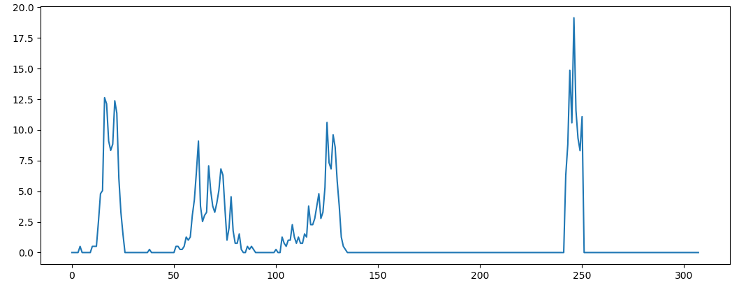
2. Visual VFH features

PCLHistogramVisualization class can be used in PCL to visualize. There are many choices in python environment. Below, use Matplotlib to draw.

# Draw histogram using matplotlib
plt.plot(vfhs.histogram[0])
plt.show()

Reference:( 1 , 2 ) http://www.willowgarage.com/sites/default/files/Rusu10IROS.pdf

6, Descriptor based on moment of inertia and eccentricity (bug)

In this tutorial, we will learn how to use the pcl::MomentOfInertiaEstimation class to obtain descriptors based on eccentricity and moment of inertia. This class also allows the extraction of axis alignment and orientation bounding boxes of clouds. However, remember that the extracted OBB is not the smallest possible bounding box.

For the theoretical part, please refer to: Moment of inertia and eccentricity based descriptors
Or visit Descriptor based on moment of inertia and eccentricity

1. Code

This tutorial point cloud files: here

see 08_moment_of_inertia.py

# Load point cloud
cloud = pcl.PointCloud.PointXYZ()
reader = pcl.io.PCDReader()
reader.read("../../data/min_cut_segmentation_tutorial.pcd", cloud)

print(cloud.size())

feature_extractor = pcl.features.MomentOfInertiaEstimation.PointXYZ()
feature_extractor.setInputCloud(cloud)
feature_extractor.compute()

moment_of_inertia = pcl.vectors.Float()
eccentricity = pcl.vectors.Float()

min_point_AABB = pcl.point_types.PointXYZ()
max_point_AABB = pcl.point_types.PointXYZ()
min_point_OBB = pcl.point_types.PointXYZ()
max_point_OBB = pcl.point_types.PointXYZ()
position_OBB = pcl.point_types.PointXYZ()

rotational_matrix_OBB = np.zeros((3, 3), np.float)
major_value, middle_value, minor_value = 0.0, 0.0, 0.0
major_vector = np.zeros((3, 1), np.float)
middle_vector = np.zeros((3, 1), np.float)
minor_vector = np.zeros((3, 1), np.float)
mass_center = np.zeros((3, 1), np.float)

feature_extractor.getMomentOfInertia(moment_of_inertia)
feature_extractor.getEccentricity(eccentricity)
feature_extractor.getAABB(min_point_AABB, max_point_AABB)
feature_extractor.getEigenValues(major_value, middle_value, minor_value)    # The last three lines don't seem to work. Functions that use numpy arrays as parameters directly seem to have this problem.
feature_extractor.getEigenVectors(major_vector, middle_vector, minor_vector)
feature_extractor.getMassCenter(mass_center)



viewer = pcl.visualization.PCLVisualizer('3D Viewer')
viewer.setBackgroundColor(0.0, 0.0, 0.0)
viewer.addCoordinateSystem(1.0)
viewer.initCameraParameters()
viewer.addPointCloud(cloud, 'simple cloud')
viewer.addCube(min_point_AABB.x, max_point_AABB.x, min_point_AABB.y, max_point_AABB.y,
               min_point_AABB.z, max_point_AABB.z, 1.0, 1.0, 0.0, 'AABB')
viewer.setShapeRenderingProperties(5, 1, 'AABB')  # Point clouds are represented by wireframes

position = np.array([[position_OBB.x], [position_OBB.y], [position_OBB.z]],
                    np.float)
quat = pclpy.pcl.vectors.Quaternionf()
viewer.addCube(position, quat, max_point_OBB.x - min_point_OBB.x,
               max_point_OBB.y - min_point_OBB.y, max_point_OBB.z - min_point_OBB.z, "OBB")
viewer.setShapeRenderingProperties(5, 1, "OBB")

center = pcl.point_types.PointXYZ()
center.x, center.y, center.z = mass_center[0], mass_center[1], mass_center[2]

x_axis = pcl.point_types.PointXYZ()
x_axis.x, x_axis.y, x_axis.z = major_vector[0] + mass_center[0],\
                               major_vector[1] + mass_center[1],\
                               major_vector[2] + mass_center[2]

y_axis = pcl.point_types.PointXYZ()
y_axis.x, y_axis.y, y_axis.z = middle_vector[0] + mass_center[0],\
                               middle_vector[1] + mass_center[1],\
                               middle_vector[2] + mass_center[2]

z_axis = pcl.point_types.PointXYZ()
z_axis.x, z_axis.y, z_axis.z = minor_vector[0] + mass_center[0], \
                               minor_vector[1] + mass_center[1], \
                               minor_vector[2] + mass_center[2]
viewer.addLine(center, x_axis, 1.0, 0.0, 0.0,  "major eigen vector")
viewer.addLine(center, y_axis, 0.0, 1.0, 0.0, "middle eigen vector")
viewer.addLine(center, z_axis, 0.0, 0.0, 1.0, "minor eigen vector")

while not viewer.wasStopped():
    viewer.spinOnce(10)

2. Description

Now let's look at the purpose of this code. The first few lines are omitted because they are obvious.

# Load point cloud
cloud = pcl.PointCloud.PointXYZ()
reader = pcl.io.PCDReader()
reader.read("../../data/min_cut_segmentation_tutorial.pcd", cloud)

Just load the cloud from the. pcd file.

feature_extractor = pcl.features.MomentOfInertiaEstimation.PointXYZ()
feature_extractor.setInputCloud(cloud)
feature_extractor.compute()

This is an instantiation of the PCL:: momentofinitiaestimation class. Then we set up the input point cloud and start the calculation process.

moment_of_inertia = pcl.vectors.Float()
eccentricity = pcl.vectors.Float()

min_point_AABB = pcl.point_types.PointXYZ()
max_point_AABB = pcl.point_types.PointXYZ()
min_point_OBB = pcl.point_types.PointXYZ()
max_point_OBB = pcl.point_types.PointXYZ()
position_OBB = pcl.point_types.PointXYZ()

rotational_matrix_OBB = np.zeros((3, 3), np.float)
major_value, middle_value, minor_value = 0.0, 0.0, 0.0
major_vector = np.zeros((3, 1), np.float)
middle_vector = np.zeros((3, 1), np.float)
minor_vector = np.zeros((3, 1), np.float)
mass_center = np.zeros((3, 1), np.float)

This is all the necessary variables we need to declare to store descriptors and bounding boxes.

feature_extractor.getMomentOfInertia(moment_of_inertia)
feature_extractor.getEccentricity(eccentricity)
feature_extractor.getAABB(min_point_AABB, max_point_AABB)
feature_extractor.getEigenValues(major_value, middle_value, minor_value)    # The last three lines don't seem to work. Functions that use numpy arrays as parameters directly seem to have this problem.
feature_extractor.getEigenVectors(major_vector, middle_vector, minor_vector)
feature_extractor.getMassCenter(mass_center)

Get descriptors and other properties.

Note that the three functions getEigenValues(), getEigenVectors(), getMassCenter() do not seem to work. Functions that use numpy array as parameters directly seem to have this problem, which has also been encountered when calculating the centroid in the previous examples.

Therefore, in fact, this tutorial only visualizes AABB, but cannot realize OBB temporarily. There is time for follow-up. You can use numpy to realize it.

viewer = pcl.visualization.PCLVisualizer('3D Viewer')
viewer.setBackgroundColor(0.0, 0.0, 0.0)
viewer.addCoordinateSystem(1.0)
viewer.initCameraParameters()
viewer.addPointCloud(cloud, 'simple cloud')
viewer.addCube(min_point_AABB.x, max_point_AABB.x, min_point_AABB.y, max_point_AABB.y,
               min_point_AABB.z, max_point_AABB.z, 1.0, 1.0, 0.0, 'AABB')
viewer.setShapeRenderingProperties(5, 1, 'AABB')  # Point clouds are represented by wireframes

Create a class instance that PCLVisualizer uses to visualize the results. Here, we also added cloud and AABB for visualization. We set the rendering properties to display the cube with wireframe, because the solid cube is used by default.

reference resources setShapeRenderingProperties() parameter

position = np.array([[position_OBB.x], [position_OBB.y], [position_OBB.z]],
                    np.float)
quat = pclpy.pcl.vectors.Quaternionf()
viewer.addCube(position, quat, max_point_OBB.x - min_point_OBB.x,
               max_point_OBB.y - min_point_OBB.y, max_point_OBB.z - min_point_OBB.z, "OBB")
viewer.setShapeRenderingProperties(5, 1, "OBB")

The visualization of OBB is slightly more complex. So here we create a quaternion from the rotation matrix, set the OBB position and pass it to the visualizer.

Here, the rotation matrix to quaternion has not been realized.

center = pcl.point_types.PointXYZ()
center.x, center.y, center.z = mass_center[0], mass_center[1], mass_center[2]

x_axis = pcl.point_types.PointXYZ()
x_axis.x, x_axis.y, x_axis.z = major_vector[0] + mass_center[0],\
                               major_vector[1] + mass_center[1],\
                               major_vector[2] + mass_center[2]

y_axis = pcl.point_types.PointXYZ()
y_axis.x, y_axis.y, y_axis.z = middle_vector[0] + mass_center[0],\
                               middle_vector[1] + mass_center[1],\
                               middle_vector[2] + mass_center[2]

z_axis = pcl.point_types.PointXYZ()
z_axis.x, z_axis.y, z_axis.z = minor_vector[0] + mass_center[0], \
                               minor_vector[1] + mass_center[1], \
                               minor_vector[2] + mass_center[2]
viewer.addLine(center, x_axis, 1.0, 0.0, 0.0,  "major eigen vector")
viewer.addLine(center, y_axis, 0.0, 1.0, 0.0, "middle eigen vector")
viewer.addLine(center, z_axis, 0.0, 0.0, 1.0, "minor eigen vector")

Feature vector visualization.

3. Operation

Run code:

After entering the folder where the code is located, enter

python 08_moment_of_inertia.py

Only AABB results.

reference resources: https://pcl.readthedocs.io/projects/tutorials/en/latest/index.html#features