
Article directory
Preparation
-
Before the beginning of the text, I will introduce the Tensorflow environment I use. It is highly recommended to use Anaconda for Mac or Windows. Most of the commonly used packages are integrated in it, and it is not recommended to match it by myself.
-
I choose pycharms as the compilation environment. There are two official versions: Community (free version) and Professional (charging version). They take what they need from each other ~ ~ of course, check whether several necessary packages are installed: Pandas, Numpy, Matplotlib, tensorflow (CPU version only tensorflow). In short, the installation method =.
- Mac environment: input PIP install panda, numpy, matplotlib, tensorflow respectively in the terminal
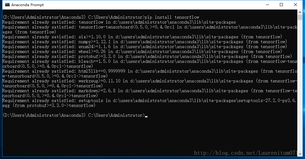
- Windows 10 environment: it is recommended to open an Anaconda prompt in anaconda, which is similar to the terminal. Input the uplink command
Important concepts
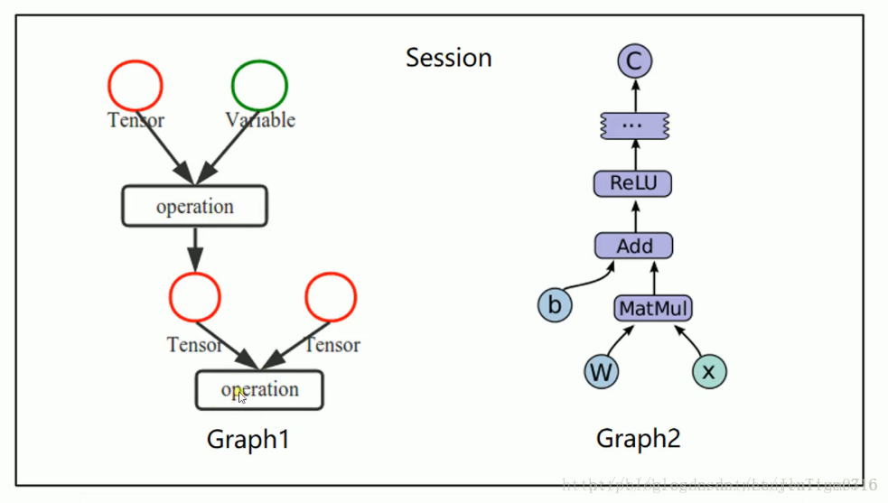
Graph and Session
- In the figure above, each circle of Graph1 is called OP (operator). The meaning of Graph is to describe the whole Graph (define calculation)
- Perform calculations in Graph in Session
Computation flow
- Data preparation
- Prepare the placeholder
- Initialization parameters / weights
- Calculate forecast results
- Calculate loss value
- Initialize optimizer
- Specify the number of iterations and execute graph in the session
Data preparation
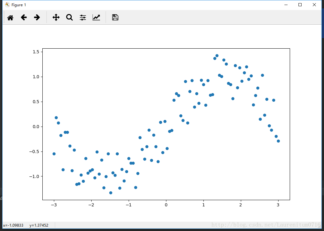
This data is generated by ourselves. We generate 100 points in [- 3, 3], and use sine function plus random noise
import numpy as np
import tensorflow as tf
import matplotlib.pyplot as plt

n_observations = 100
xs = np.linspace(-3, 3, n_observations)
ys = np.sin(xs) + np.random.uniform(-0.5, 0.5, n_observations)
plt.scatter(xs, ys)
plt.show()
Prepare the placeholder
The placeholder stores the data used for training and passes it into the placeholder in the form of a dictionary (to be used later)
X = tf.placeholder(tf.float32, name='X')
Y = tf.placeholder(tf.float32, name='Y')
Initialization parameters / weights
In linear regression, y = wx + b is used for fitting. Here, two variables w and b are constructed. tf.Variable is a class. The initialized object can have multiple OPS, and here it is initialized as a random number
W = tf.Variable(tf.random_normal([1]), name='weight')
B = tf.Variable(tf.random_normal([1]), name='bias')
Calculate forecast results
y = wx + b
Y_pred = tf.add(tf.multiply(X, W), B)
Calculate loss value
loss = tf.square(Y - Y_pred, name='loss')
Initialize optimizer
Use the most conventional gradient descent function to minimize the value of the loss function. Congratulations on the completion of drawing the whole picture, that is, defining all calculations. Next, we start to perform calculations
learning_rate = 0.01
optimizer = tf.train.GradientDescentOptimizer(learning_rate).minimize(loss)
Specify the number of iterations and execute graph in the session
These two sentences are extremely important. Variables need to be initialized before reading and writing (assigning) operations can be performed
n_sample = xs.shape[0]
init = tf.global_variables_initializer()

with tf.Session() as sess:
    sess.run(init)

    for i in range(50):
        total_loss = 0
        for x, y in zip(xs, ys):
            __, l = sess.run([optimizer, loss], feed_dict={X: x, Y: y})
            total_loss += l
        if i % 5 == 0:
            print('Epoch{0}:{1}'.format(i, total_loss/n_sample))

    W, B = sess.run([W, B])

plt.scatter(xs, ys)
plt.plot(xs, xs*W + B)
plt.show()
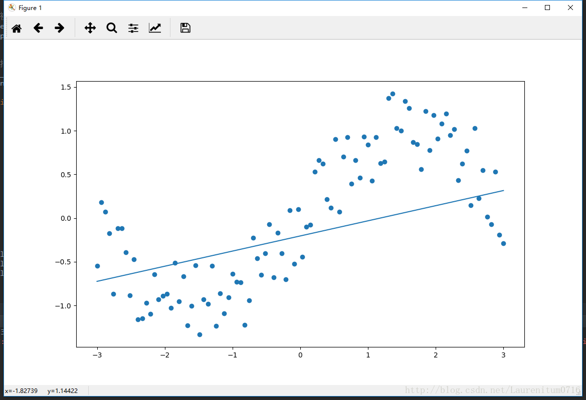
Operation result
After 50 iterations, it can be found that the loss value does not continue to decrease, because linear quasi merging is not suitable for sinusoidal functions. This example is just to help you build a Tensorflow framework. In the next phase, the polynomial regression will be modified on this framework to produce different effects
Complete code
import numpy as np
import tensorflow as tf
import matplotlib.pyplot as plt


#Data preparation
n_observations = 100
xs = np.linspace(-3, 3, n_observations)
ys = np.sin(xs) + np.random.uniform(-0.5, 0.5, n_observations)
#plt.scatter(xs, ys)
#plt.show()


#Prepare the placeholder
X = tf.placeholder(tf.float32, name='X')
Y = tf.placeholder(tf.float32, name='Y')


#Initialization parameters / weights
W = tf.Variable(tf.random_normal([1]), name='weight')
B = tf.Variable(tf.random_normal([1]), name='bias')


#Calculate forecast results
Y_pred = tf.add(tf.multiply(X, W), B)

#Calculate loss value
loss = tf.square(Y - Y_pred, name='loss')

#Initialize optimizer
learning_rate = 0.01
optimizer = tf.train.GradientDescentOptimizer(learning_rate).minimize(loss)


#Specify the number of iterations and execute graph in the session
n_sample = xs.shape[0]
init = tf.global_variables_initializer()

with tf.Session() as sess:
    sess.run(init)

    for i in range(50):
        total_loss = 0
        for x, y in zip(xs, ys):
            __, l = sess.run([optimizer, loss], feed_dict={X: x, Y: y})
            total_loss += l
        if i % 5 == 0:
            print('Epoch{0}:{1}'.format(i, total_loss/n_sample))

    W, B = sess.run([W, B])

plt.scatter(xs, ys)
plt.plot(xs, xs*W + B)
plt.show()


